5. Conditional and Repetitive Execution¶ Open the notebook in Colab
(C) Copyright Notice: This chapter is part of the book available athttps://pp4e-book.github.io/and copying, distributing, modifying it requires explicit permission from the authors. See the book page for details:https://pp4e-book.github.io/
Many circumstances require the execution to change its flow based on the truth value of a condition or to repeat a set of steps for a number of items or until a condition is not true any more. These two kinds of actions are very crucial components of programming solutions and Python provides several alternatives for them. As we are going to see in this chapter, some of these alternatives are compound statements, i.e. they include other statements as part of the statement, whereas others are expressions.
5.1. Conditional execution
Asking (mostly) mathematical questions that have Boolean type answers and taking some actions (or not) based on the Boolean answers are crucial tools in designing algorithms. This is so vital that there is no single programming language that does not provide conditional execution.
5.1.1. if statement
The syntax of the conditional (if) statement is
if \(\boxed{\color{red}{Boolean\ expression\strut\ }}\) :
\(\boxed{\color{red}{Statement\strut\ }}\)
The semantics is obvious. If the
\(\color{red}{Boolean\ expression}\) evaluates to True, then the
\(\color{red}{Statement}\) is carried out; otherwise
\(\color{red}{Statement}\) is not executed.
>>> if 5 > 2: print("Hurray")
Hurray
>>> if 2 > 5: print("No I will not believe that !")
We observe that the Boolean expression in the last example evaluates to
False and hence the statement with the print function is not carried
out.
How to group statements?
It is quite often that we want to do more then one action instead of executing a single statement. As a general syntax rule of Python:
switch to a new line,
indent by one tab,
write your first statement to be executed,
switch to the next line,
indent the same amount (usually your Python-aware editor will do it for you)
write your second statement to be executed,
and so on…
To finish this writing task, and presumably enter a statement which is not part of the group action, just do not intend.
It is very very important that the statements that are part of the if part have the same amount and type of whitespace. E.g. if the first statement has 4 spaces, all following statements in the if statement need to start with 4 spaces. If it is a tab character, all following statements in the if statement need to start with a tab character. Since these whitespaces are not visible, it is very easy to make mistakes and get annoying errors from the interpreter. To avoid this, we strongly recommend you to choose a style of indentation (e.g. 4 whitespaces or a single tab) and stick to it as a programming style.
Here is an example:
>>> if 5 > 2:
...     print(7*6)
...     print("Hurray")
...     x = 6
42
Hurray
>>> print(x)
6
The >>> as well as ... prompts appear when you sit in front of
the interpreter. When you type your programs into a file and then run
them, of course they will not show up. If you type in these small
programs (we call them snippets) just ignore the >>> and ...
from the examples, as follows:
if 5 > 2:
  print(7*6)
  print("Hurray")
  x = 6
print(x)
42
Hurray
6
As you continue practicing programming, you will soon come across a need
to be able to define actions that should be carried out in case a
Boolean expression turns out to be False. If it were not provided,
we would have to ask the same question again, but this time negated:
>>> if x == 6: print("still it is six")
>>> if not (x == 6): print("it is no more six")
One of them will certainly fire (be true). Although this is a feasible
solution, there is a more convenient way: We can combine the two parts
into one if-else statement with the following syntax:
if \(\boxed{\color{red}{Boolean\ expression\strut\ }}\) :
\(\boxed{\color{red}{Statement\strut\ }}\)
else : \(\boxed{\color{red}{Statement\strut\ }}\)
Making use of the else part, the last example would be written as:
>>> if x == 6: print("still it is six")
... else: print("it is no more six")
Of course, using multiple statements in the if part or the else
part is possible by intending them to the same level.
5.1.2. Exercise
In the following code cell, you are expected to insert a couple of lines so that the output is always the absolute value of N (try the program for various values of N by altering the right-hand side of the assignment):
N = -100   # Feel free to change this to any numerical value #

# @TODO type in your code that changes the content of N to its absolute value, below this line

# @TODO print the result
5.1.3. Nested if statements
It is quite possible to nest if-else statements: i.e. combine
multiple if-else statements within each other. There is no practical
limit to the depth of nesting. This enables us to code a structure,
called a decision tree. A decision tree is a set of binary questions &
answers where at every case of an answer either a new question is asked
or an action is carried out. Fig. 5.1.1 displays such
a decision tree for forecasting rain based on the temperature, wind
and air pressure values.
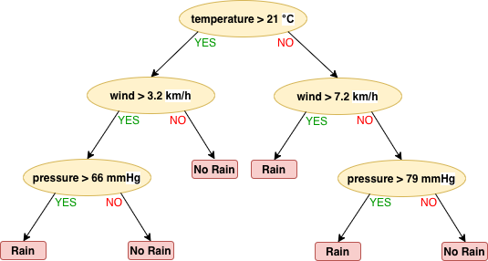
Fig. 5.1.1 An example decision tree.
The tree in Fig. 5.1.1 can be coded as nested
if-else statements:
if temperature > 21:
     if wind > 3.2:
          if pressure > 66: rain = True
          else: rain = False
     else: rain = False
else:
     if wind > 7.2: rain = True
     else:
          if pressure > 79: rain = True
          else: rain = False
Sometimes the else case contains another if which has an
else of its own. And this ladder goes on. For such a case, elif
serves as a combined keyword for the else if action, as follows:
if \(\boxed{\color{red}{Boolean\ expression_1\strut}}\) :
\(\boxed{\color{red}{Statement_1\strut}}\)
elif \(\boxed{\color{red}{Boolean\ expression_2\strut}}\) :
\(\boxed{\color{red}{Statement_2\strut}}\)
\(\;\;\mathbf{\vdots}\)
elif \(\boxed{\color{red}{Boolean\ expression_n\strut}}\) :
\(\boxed{\color{red}{Statement_n\strut}}\)
else : \(\boxed{\color{red}{Statement_{otherwise}\strut}}\)
The flowchart in Fig. 5.1.2 explains the semantics of the
if-elif-else combination.
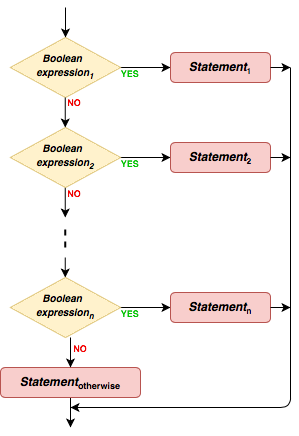
Fig. 5.1.2 The semantics of the if-elif-else combination.
There is no restriction on how many elif statements are used.
Furthermore, the presence of the last statement (the else) is
optional.
5.1.4. Practice
Let us assume that you have a value assigned to a variable x. Based
on this value, a variable s is going to be set as:
It is convenient to make use of an if-elif-else structure:
#@TODO Assign a value to x
x = 10

if x < 1: s = (x+1)**2
elif x < 10: s = x-0.5
elif x < 100: s = (x+0.5)**0.5
else: s = 0

print("s is: ", s)
s is: 3.24037034920393
5.1.5. Conditional expression
The if statement does not return a value. As said, that is so for
all statements. They do not have a value of their own. A non-statement
alternative that has a return value is the conditional expression.
It also uses the if and else keywords. This time if is not
at the start of a statement, but following a value. Here is the syntax:
\(\boxed{\color{red}{ expression_{YES}\strut\ }}\) if
\(\boxed{\color{red}{Boolean\ expression\strut\ }}\) else
\(\boxed{\color{red}{ expression_{NO}\strut\ }}\)
This whole structure is an expression. It yields a value. So, it can be used in any place an expression is allowed to be used. It is evaluated as follows:
First the \(\color{red}{Boolean\ expression}\) is evaluated.
If the outcome is
Truethen \(\color{red}{expression_{YES}}\) is evaluated and used as value (\(\color{red}{expression_{NO}}\) is left untouched).If the outcome is
Falsethen \(\color{red}{expression_{NO}}\) is evaluated and used as value (\(\color{red}{expression_{YES}}\) is left untouched).
Though it is not compulsory, it is wise to use conditional expression enclosed in parenthesis to prevent wrong sub-expression groupings.
Let us look at an example:
>>> x = -34.1905
>>> y = (x if x > 0 else -x)**0.5
>>> print(y)
5.84726431761
As you have observed, y is assigned the value
\(\sqrt{{\scriptsize|\mathtt{x}|}}\). For code readability, it is
strongly advisable not to nest conditional expressions. Instead,
restructure your coding into nested if-else statements (by making
use of intermediate variables).
5.2. Repetitive execution
Repeating a sequence of instructions over-and-over is a programming ingredient which is used frequently. This action is called iteration or loop.
We use iteration
to systematically deal with all possible cases or all elements of a collection, or
to jump from one case to another as a function of the previous case.
The repetition of a sequence of instructions is carried out either for a known number of times or until a criterion is met.
Iteration examples:
Computing letter grades of a class (Type I, for all students).
Finding the shortest path from city A to city B in a map (Type II).
Root finding by Newton-Raphson method (Type II).
Finding darkest and brightest point(s) in a image (Type I, for all pixels).
Computing a function value using Taylor’s expansion (Type I).
Computing the next move in a chess game (Type II).
Obtaining the letter frequency of a text (Type I, for all letters).
Python provides two statements for iteration. Namely, while and
for. for is used mostly for (Type I) iterations whereas
while is used for both types.
5.2.1. while statement
The syntax of while resembles the synax of the if statement:
while \(\boxed{\color{red}{Boolean\ expression\strut\ }}\) :
\(\boxed{\color{red}{Statement\strut\ }}\)
It is certainly possible to have a statement group subject to the
while, as it was with the if statement. The semantics can be
expressed as the flowchart in Fig. 5.2.1:
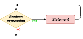
Fig. 5.2.1 The flowchart illustrating how a while statement is executed.
Later in this chapter, when we have introduced the for statement as
well, we will consider some special statements (break and
continue) that are allowed only under the scope of a while or
for and are capable of altering the execution flow (to some limited
extent).
Since a while statement is a statement, it can be part of another while statement (or any other compound statement):
while <condition-1>:
   statement-1
   statement-2
   ...
   while <condition-2>:
      statement-inner-1
      statement-inner-2
      ...
      statement-inner-M
   ... # statements after the second while
   statement-N
Of course, there is no practical limit on the nesting level.
Let us look at several examples below to illustrate these concepts.
5.2.2. Examples with while statement
Example 1: Finding Average of Numbers in a List
Let’s say we have a list of numbers and we are asked to find their average. To make things easier to follow, let us start with the mathematical definition:
where \(L_i\) is the \(i\)th number in the list which contains \(N\) numbers.
Let us see the algorithm before implementing a solution in Python (note that, in the equation, indexing started with 1 – compare this with the following):
Input: A list L that includes N numbers
Output: avg, which holds the average of numbers in L

Step 1: Initialize a sum variable with value 0
Step 2: Initialize an index variable, i, with value 0
Step 3: While i is less than N, Execute Steps 4-5
Step 4:     sum = sum + L[i]
Step 5:     i = i + 1
Step 6: avg = sum/N
Before we proceed with the Python implementation, make sure that you have understood the algorithm. The best way to make sure that is to take a pen & paper and go through each step while keeping a track of the variables, as if you are the computer.
Here is the implementation in Python:
# L: the list of numbers
# @TODO: Change the list and check if the code works
L = [10, -4, 4873, -18]
N = len(L)

sum = 0            # Step 1
i = 0              # Step 2

while i < N:       # Step 3
  sum = sum + L[i] # Step 4
  i = i + 1        # Step 5

avg = sum / N      # Step 6
print(avg)
1215.25
Have you noticed how close the Python code is to the algorithm? Python’s principles for keeping things simple makes it so much easier to write that it can be very close to the pseudo-code.
Example 2: Standard Deviation
Now, let us look at a highly related problem, that of calculating the standard deviation. Standard deviation can be formally defined as follows:
The extension of the previous example is rather straightforward therefore but we will write it down nonetheless since these are your first iterative examples.
L = [10, 20, 30, 40]
N = len(L)

# CALCULATE THE AVG FIRST (COPY-PASTE FROM THE FIRST EXAMPLE)
sum = 0
i = 0

while i < N:
  sum = sum + L[i]
  i = i + 1

avg = sum / N

# CALCULATE THE STD NOW
sum = 0
i = 0

while i < N:
  sum = sum + (L[i] - avg)**2
  i = i + 1

std = (sum / N)**0.5

print("Avg & Std of the list are: ", avg, std)
Avg & Std of the list are: 25.0 11.180339887498949
Exercise
Write down the algorithm that we used in this Python code as a pseudo-code.
Example 3: Factorial Factorial of a number, denoted by \(n!\), is an important mathematical construct that we frequently use while formulating our solutions. \(n!\) can be defined formally as:
Let us first write down the algorithm:
Input: n
Output: n_factorial

Step 1: If n is zero or negative, n_factorial is 1. Return n_factorial and exit
Step 2: Initialize n_factorial with 1
Step 3: Initialize an index variable, i, with 1
Step 4: While i <= n, Execute Steps 5 and 6:
Step 5:     n_factorial = n_factorial * i
Step 6:     i = i + 1
Step 7: The result is n_factorial
which can be implemented in Python as follows:
# Let us choose an n value:
n = 5

if n <= 0: n_factorial = 1  # Step 1
elif n > 0:                # Steps 2-6
  n_factorial = 1          # Step 2
  i = 1                    # Step 3
  while i <= n:            # Step 4
    n_factorial *= i       # Step 5
    i += 1              # Step 6

print("n! is ", n_factorial)
n! is 120
Exercise
Modify our factorial implementation such that variable i starts from
n.
Example 4: Computing Sine with Taylor Expansion
Let us assume we want to compute \(\sin(x)\), for a given value of \(x\), up to a given precision. This is just for the sake of having an understandable example. Actually today’s CPUs have embedded math coprocessors that do this at microcode level. We will not use this convenience and do the computation ourselves.
The computation of many analytic functions are performed using the Taylor series expansion. The Taylor series expansion of \(\sin(x)\) around zero is:
which could also be written as:
Let us implement this. We will use the factorial example as a nested iteration. The outer iteration runs over the terms in the summation, and continues until a term becomes too small (\(|term| < \epsilon\), where \(\epsilon\) is a small value, e.g. \(10^{-12}\)).
epsilon = 1.0E-12
x = 3.14159265359/4.0   # i.e. pi/4 (45 degrees in radians)
result = 0.0
k = 0
term = 2*epsilon    #just a trick to bypass the first test
while abs(term) > epsilon:
    # Calculate the denominator - i.e. (2k+1)!
    factorial = i = 1
    while i <= 2*k+1:
      factorial *= i
      i += 1

    # Now calculate the term
    term = (((-1)**k) / factorial) * (x**(2*k+1))

    result += term
    k += 1
2*k+1 is computed several times. Actually, do we need 2*k+1
at all? * It uses factorial computation which does not make use of
its preceeding computations. For example \(9!\) is actually
\(9\times 8 \times 7!\). But it is computed as
\(2 \times 3 \times 4 \times 5 \times 6 \times 7 \times 8 \times 9\).
Therefore, there is significant inefficiency regarding the use of
factorial in the nested iteration. * Similar to the inefficiency with
the factorial computation, the computation of \(x^{(n+2)}\) does
not make use of the already computed \(x^n\) value.Let us investigate the proportionality of two consecutive terms \((k=n)\) and \((k=n+1)\):
This is interesting because it suggests us a relatively faster way to compute the next term in the series. We do not have to compute \(x^n\) for each new term that we are going to add. We also discover that there is nothing magical about \((2n+1)\). It can simply be called as \((d \equiv 2n+1)\) which increments by 2 for each consecutive term. Then we have
Now, let us see the more efficient implementation in action:
epsilon = 1.0E-12
x = 3.14159265359/4.0   # i.e. pi/4 (45 degrees in radians)
x_square = x*x
term = x
result = term
d = 1    #  2*n+1
while abs(term) > epsilon:
    term *= -x_square/((d+1)*(d+2))
    result += term
    d += 2

print("sin(x) [Ours] is: ", result)

# Compare this with the CPU-implemented version
from math import *
print("sin(x) [CPU ] is: ", sin(x))
sin(x) [Ours] is:  0.707106781186584
sin(x) [CPU ] is:  0.7071067811865841
5.2.3. for statement
The syntax of the for statement is:
for \(\boxed{\color{red}{Variable\strut\ }}\) in
\(\boxed{\color{red}{Iterator\strut\ }}\) :
\(\boxed{\color{red}{Statement\strut\ }}\)
An iterator is an object that provides a countable number of values on demand. It has an internal mechanism that responds to three requests:
Reset (initialize) it to the start.
Respond to the “Are we at the end?” question.
Provide the next value in line.
The for statement is a mechanism that allows traversing all values
provided by an \(\color{red}{Iterator}\), one-by-one assigning them
to a \(\color{red}{Variable}\) and then executiong a given
\(\color{red}{Statement}\).
The semantics of the for statement is displayed in Fig. 5.2.2:
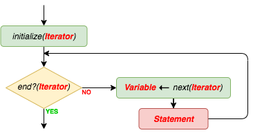
Fig. 5.2.2 The flowchart illustrating how a for statement is executed.
What iterators do we have?
All containers are also iterators (strings, lists, dictionaries, sets).
The built-in function
rangereturns an iterator that generates a sequence of integers, starting from 0 (default), and increments by 1 (default), and stops before a given number:
range(\(\color{red}{start}\), \(\color{red}{stop}\),
\(\color{red}{step}\))
Parameter |
Opt./Req. |
Default |
Description |
|
|---|---|---|---|---|
start |
Optional |
0 |
An integer specifying the start value. |
|
stop |
Required |
An integer specifying the stop value (stop value will not be taken) |
||
step |
Optional |
1 |
An integer specifying the in crementation. |
A user-defined iterator. Since this is an introductory book, we will not cover how this is done.
5.2.4. Examples with for statement
Example 1: Words Starting with Vowels and Consonants
Let us split a list of words into two lists: those that start with a vowel and those that start with a consonant.
mixed = ["lorem","ipsum","dolor","sit","amet,","consectetur","adipiscing","elit","sed","do","eiusmod","tempor","incididunt","ut","labore","et","dolore","magna","aliqua"]
vowels = []
consonants = []
for word in mixed:
    if word[0] in ['a','e','i','o','u']: vowels += [word]
    else: consonants += [word]

print("Starting with consonant:", consonants)
print("Starting with vowel:", vowels)
Starting with consonant: ['lorem', 'dolor', 'sit', 'consectetur', 'sed', 'do', 'tempor', 'labore', 'dolore', 'magna']
Starting with vowel: ['ipsum', 'amet,', 'adipiscing', 'elit', 'eiusmod', 'incididunt', 'ut', 'et', 'aliqua']
Exercise
Write this solution in pseudo-code.
Example 2: Run-length Encoding
Run-length encoding is a compression technique for data that repeats
itself contiguously. Images bear such data: For example, a clear sky
portion is actually rows of ‘blue’. In the example below, we investigate
a string for consequent character occurrences: If found, repetitions are
coded as a list of [character, repetition count].
"aaaaaaxxxxmyyyaaaassssssssstttuivvvv" gets encoded
as:[a',6],['x',4],'m',['y',3],['a',4],['s',9],['t',3],'u','i',['v',4]].text = "aaaaaaxxxxmyyyaaaassssssssstttuivvvv"
code_list = []
last_character = text[0]
count = 1
# Go over each character except for the first
for curr_character in text[1:]:
# If curr_character is equal to last_character, we found a duplicate
if last_character == curr_character:
count += 1
else:
# We have finished a sequence of same characters: Save the count and
# reinitialize last_character and count accordingly
code_list += [last_character if count==1 else [last_character, count]]
count = 1
last_character = curr_character
# handle the last_character here:
code_list += [last_character if count==1 else [last_character,count]]
print(code_list)
[['a', 6], ['x', 4], 'm', ['y', 3], ['a', 4], ['s', 9], ['t', 3], 'u', 'i', ['v', 4]]
Exercise
Modify this code such that it removes consecutive duplicate characters.
In other words, "aaaabbbcdd" should be reduced to "abcd".
Example 3: Permutations
Permutations are keys to shuffling a sequence of data. Permutations can be denoted in various forms. One way is to give an order list: The \(i^{\mathrm{th}}\) element of the list stores the old position where the \(i^{\mathrm{th}}\) element of the new sequence will come from. In our implementation counting starts from 0 (zero).
word_list = ["he","came","home","late","yesterday"]
permutation = [4,3,2,0,1]
length = len(permutation)
new_list = [None]*length

for i in range(length):
    new_list[i] = word_list[permutation[i]]

print(new_list)
['yesterday', 'late', 'home', 'he', 'came']
Example 4: List Split
In the example below the first element of the list is taken and the rest is split into two lists: Those that are smaller than the first element, and those that are not.
list_to_split = [42, 59, 53, 84, 43, 8, 75, 34, 40, 89, 29, 15, 51, 6, 90, 32, 58, 77, 4, 24]
list_smaller = []
list_not_smaller = []

for x in list_to_split[1:]:
    if x < list_to_split[0]: list_smaller += [x]
    else: list_not_smaller += [x]

print("list head was.        :",list_to_split[0])
print("smaller than head     :", list_smaller)
print("not smaller than head :", list_not_smaller)
list head was.        : 42
smaller than head     : [8, 34, 40, 29, 15, 6, 32, 4, 24]
not smaller than head : [59, 53, 84, 43, 75, 89, 51, 90, 58, 77]
Example 5: Dot Product
A frequently used operation with vectors is the dot product between two vectors, e.g. \(\mathbf{u}\) and \(\mathbf{v}\):
where the vectors have \(n\) elements each. Let us implement this in Python:
# Define the vectors (as lists)
u = [1, 2, 4, 10]
v = [10, 4, 2, 1]
n = len(u)
dot_prod = 0

if n != len(v): print("Sizes don't match!")
else:
  for i in range(n):
    dot_prod += u[i] * v[i]
  print("u . v is: ", dot_prod)
u . v is: 36
Exercise
Implement dot product between two vectors using a while statement.
Example 6: Angle between Two Vectors
The angle between two vectors \(\mathbf{u}\) and \(\mathbf{v}\) is closely related to their dot product:
where \(\theta\) is the angle between the vectors, and \(||\cdot||\) denotes the norm of a vector:
The angle can be derived from these as follows:
Let us implement this:
from math import sqrt, acos

# Define two vectors that have 90deg (pi/2) between them
u = [1, 0, 0]
v = [0, 1, 0]
n = len(u)

if n != len(v):
  print("Sizes don't match!")

else:
  # Calculate dot product & norms
  dot_prod = u_norm_sum = v_norm_sum = 0
  for i in range(n):
    dot_prod   += u[i] * v[i]
    u_norm_sum += u[i] ** 2
    v_norm_sum += v[i] ** 2

  u_norm = sqrt(u_norm_sum)
  v_norm = sqrt(v_norm_sum)

  theta = acos(dot_prod / u_norm * v_norm)

  print("angle between u and v is: ", theta)
angle between u and v is: 1.5707963267948966
Example 7: Matrix Multiplication
Our last example is matrix multiplication. As you know, a matrix \(A\) can be multipled with the matrix \(B\) if the column-count (\(m\)) of \(A\) is equal to the row-count of \(B\). The product matrix is of a size where row-count equals that of \(A\) and the column-count equals that of \(B\).
As we discussed in the previous chapter, since Python provides no two dimensional containers, but a very fexible list container, matrices are mostly represented as lists of lists each of which represent a row. For example, a \(3\times 4\) matrix:
can be represented as:
A = [[-2,3,5,-1], [0,3,10,-7], [11,0,0,-8]]
This representation is also coherent with the indexing of matrices:
\(A_{ij}\) is accessible in Python as A[i][j]. The code below
multiples two matrices, given in this representation, and prints the
result.
A = [[-2,3,5,-1], [0,3,10,-7], [11,0,0,-8]]
B = [[2,1], [-1,1], [0,4], [8,0]]

# C = A*B

# Create a result matrix with entries filled with 0 (zeros)
C = []
for i in range(len(A)):
  C += [[0] * len(B[0])]  # This is done to overcome the aliasing problem

for i in range(len(C)):
    for j in range(len(C[0])):
        for k in range(len(B)):
            C[i][j] += A[i][k]*B[k][j]

print(C)
[[-15, 21], [-59, 43], [-42, 11]]
5.2.5. continue and break statements
It is possible to alter the flow of execution in a while or for
repetition. This is almost always used in combination with statement
grouping, where a group of statements is subject to the while or
for.
Let’s assume you are executing a sequence of statements by means of
statement grouping. Somewhere in the process, without waiting for the
terminating condition to become False in a while statement or
exhausting all items in the iterator in a for statement, you decide
to terminate looping. The break statement does exactly serve this
purpose: The while (or for) is stopped immediately and the
execution continues with the statement after the while (or for).
Similarly, somewhere in the process you decide not to execute the rest
of the statements in the grouping and straight away continue with the
test. This is achieved by a continue statement usage. See
Fig. 5.2.3 and
Fig. 5.2.4 for how the continue
statement changes the flow of execution.
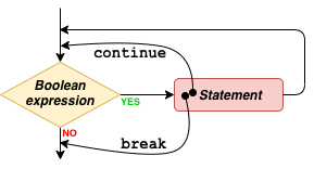
Fig. 5.2.3 How continue and break statements change execution in a
while statement.
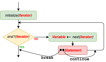
Fig. 5.2.4 How continue and break statements change execution in a
for statement.
5.2.6. Set and list comprehension
A well-known and extensively-used notation to describe a set in mathematics is the so-called ‘set-builder notation’. This is also known as set comprehension. This notation has three parts (from left-to-right):
an expression in terms of a variable,
a colon or vertical bar separator, and
a logical predicate.
Something like this:
which defines the set:
or as something more elaborate:
defining
There exists a Python notation with the same semantics both for sets and lists:
>>> [x**3 for x in range(8)]
[0, 1, 8, 27, 64, 125, 216, 343]
>>> {x**3 for x in range(8)}
{0, 1, 64, 8, 343, 216, 27, 125}
The second example, which imposes a constraint on x to be an odd
number, would be coded as:
>>> [x**3 for x in range(8) if x%2 == 1]
[1, 27, 125, 343]
>>> {x**3 for x in range(8) if x%2 == 1}
{1, 27, 125, 343}
Certainly the condition (following the if keyword) could have been
constructed as a more complex boolean expression.
The expression that can appear to the left of the for keyword can be
any Python expression and container. Here are a couple of more examples
on matrices.
print( [[0 for i in range(3)] for j in range(4)] )
print( [[1 if i==j else 0 for i in range(3)] for j in range(3)] )
print( [[(i,j) for i in range(3)] for j in range(4)] )
print( [[(i+j)%2 for i in range(3)] for j in range(4)] )
print( [[i+3*j for i in range(3)] for j in range(4)] )
[[0, 0, 0], [0, 0, 0], [0, 0, 0], [0, 0, 0]]
[[1, 0, 0], [0, 1, 0], [0, 0, 1]]
[[(0, 0), (1, 0), (2, 0)], [(0, 1), (1, 1), (2, 1)], [(0, 2), (1, 2), (2, 2)], [(0, 3), (1, 3), (2, 3)]]
[[0, 1, 0], [1, 0, 1], [0, 1, 0], [1, 0, 1]]
[[0, 1, 2], [3, 4, 5], [6, 7, 8], [9, 10, 11]]
5.3. Important Concepts
We would like our readers to have grasped the following crucial concepts and keywords from this chapter:
Conditional execution with
if,if-else,if-elif-elsestatements.Nested if statements.
Conditional expression as a form of conditional computation in an expression.
Repetitive execution with while and for statements.
Changing the flow of iterations with
breakandcontinuestatements.Set and list comprehension as a form of iterative computation in an expression.
5.4. Further Reading
“Managing the size of a problem”, Chapter 4 of “Introduction to Programming Concepts with Case Studies in Python”: https://link.springer.com/chapter/10.1007/978-3-7091-1343-1_4
5.5. Exercises
We have provided many exercises throughout the chapter, please study and answer them as well.
Implement the
whilestatement examples in Section 5.2.2 usingforstatement:Calculating the average of a list of numbers.
Calculating the standard deviation of a list of numbers.
Calculating the factorial of a number.
Taylor series expansion of sin(x).
Implement the
forstatement examples in Section 5.2.4 usingwhilestatement:Words with vowels and consonants.
Run-length encoding.
Permutation.
List split.
Matrix multiplication.
What does the variable c hold after executing the following Python code?
c = list("address")
for i in range(0, 6):
  if c[i] == c[i+1]:
      for j in range(i, 6):
          c[j] = c[j+1]
Write a Python code that removes duplicate items in a list. E.g.
[12, 3, 4, 12]should be changed to[12, 3, 4]. The order of items should not change.Write a Python code that replaces a nested list of numbers with the average of the numbers. E.g.
[[1, 3], [4, 5, 6], 7, [10, 20]]should yield[2, 5, 7, 15].Write a Python code that finds all integers dividing a given integer without a remainder. E.g. for number 21, your code should compute
[1, 3, 7].Write a Python code that converts an integer (less than 128) into binary string using a for/while statement. E.g. 21 should be represented as
00010101.Write a Python code that convers a binary string like
00010101into integer.