Preface Colab

Open the notebook in Colab

(C) Copyright Notice: This chapter is part of the book available athttps://pp4e-book.github.io/and copying, distributing, modifying it requires explicit permission from the authors. See the book page for details:https://pp4e-book.github.io/

i. About this book

a. Target audience of the book

This book is intended to be an accompanying textbook for teaching programming to science and engineering students with no prior programming expertise. This endeavour requires a delicate balance between providing details on computers & programming in a complete manner and the programming needs of science and engineering disciplines. With the hopes of providing a suitable balance, the book uses Python as the programming language, since it is easy to learn and program. Moreover, for keeping the balance, the book is formed of three parts:

• Part I: The Basics of Computers and Computing: The book starts with what computation is, introduces both the present-day hardware and software infrastructure on which programming is performed and introduces the spectrum of programming languages.

• Part II: Programming with Python: The second part starts with the basic building blocks of Python programming and continues with providing the ground formation for solving a problem in to Python. Since almost all science and engineering libraries in Python are written with an object-oriented approach, a gentle introduction to this concept is also provided in this part.

• Part III: Using Python for Science and Engineering Problems: The last part of the book is dedicated to practical and powerful tools that are widely used by various science and engineering disciplines. These tools provide functionalities for reading and writing data from/to files, working with data (using e.g. algebraic, numerical or statistical computations) and plotting data. These tools are then utilized in example problems and applications at the end of the book.

b. How to use the book

This is an ‘interactive’ book with a rather ‘minimalist’ approach: Some details or specialized subjects are not emphasized and instead, direct interaction with examples and problems are encouraged. Therefore, rather than being a ‘complete reference manual’, this book is a ‘first things first’ and ‘hands on’ book. The pointers to skipped details will be provided by links in the book. Bearing this in mind, the reader is strongly encouraged to read and interact all contents of the book thoroughly.

The book’s interactivity is thanks to Jupyter notebook. Therefore, the book differs from a conventional book by providing some dynamic content. This content can appear in audio-visual form as well as some applets (small applications) embedded in the book. It is also possible that the book asks the the reader to complete/write a piece of Python program, run it, and inspect the result, from time to time. The reader is encouraged to complete these minor tasks. Such tasks and interactions are of great assistance in gaining acquaintance with Python and building up a self-confidence in solving problems with Python.

Thanks to Jupyter notebook running solutions on the Internet (e.g. Google Colab, Jupyter Notebook Viewer), there is absolutely no need to install any application on the computer. You can directly download and run the notebook on Colab or Notebook Viewer. Though, since it is faster and it provides better virtual machines, the links to all Jupyter notebooks will be served on Colab.

ii. What is computing?

Computing is the process of inferring data from data. What is going to be inferred is defined as the task. The original data is called the input (data) and the inferred one is the output (data).

Let us look at some examples:

• Multiplying two numbers, \(X\) and \(Y\), and subtracting \(1\) from the multiplication is a task. The two numbers \(X\) and \(Y\) are the input and the result of \(X\times Y - 1\) is the output

• Recognizing the faces in a digital picture is a task. Here the input is the color values (3 integers) for each point (pixel) of the picture. The output is, as you would expect, the pixel positions that belong to faces. In other words, the output can be a set of numbers.

• The board instance of a chess game, as input, where black has made the last move. The task is to predict the best move for white. The best move is the output.

• The input is a set of three-tuples which look like <Age_of_death, Height, Gender>. The task, an optimization problem in essence, is to find out the curve (i.e. the function) that goes through these tuples in a 3D dimensional space spanned by Age, Height and Gender. As you have guessed already, the output is the parameters defining the function and an error describing how well the curve goes through the tuples.

• The input is a sentence to a chatbot. The task is to determine the sentence (the output) that best follows the input sentence in a conversation.

These examples suggest that computing can involve different types of data, either as input or output: Numbers, images, sets, or sentences. Although this variety might appear intimidating at first, we will see that, by using some ‘solution building blocks’, we can do computations and solve various problems with such a wide spectrum of data.

iii. Are all ‘computing machinery’ alike?

Certainly not! This is a common mistake a layman does. There are diverse architectures based on totally different physical phenomena that can compute. A good example is the brain of living beings, which rely on completely different mechanisms compared to the micro processors sitting in our laptops, desktops, mobile phones and calculators.

The building blocks of a brain is the neuron, a cell that has several input channels, called dendrites and a single output channel, the axon, which can branch like a tree (see Fig. 1).

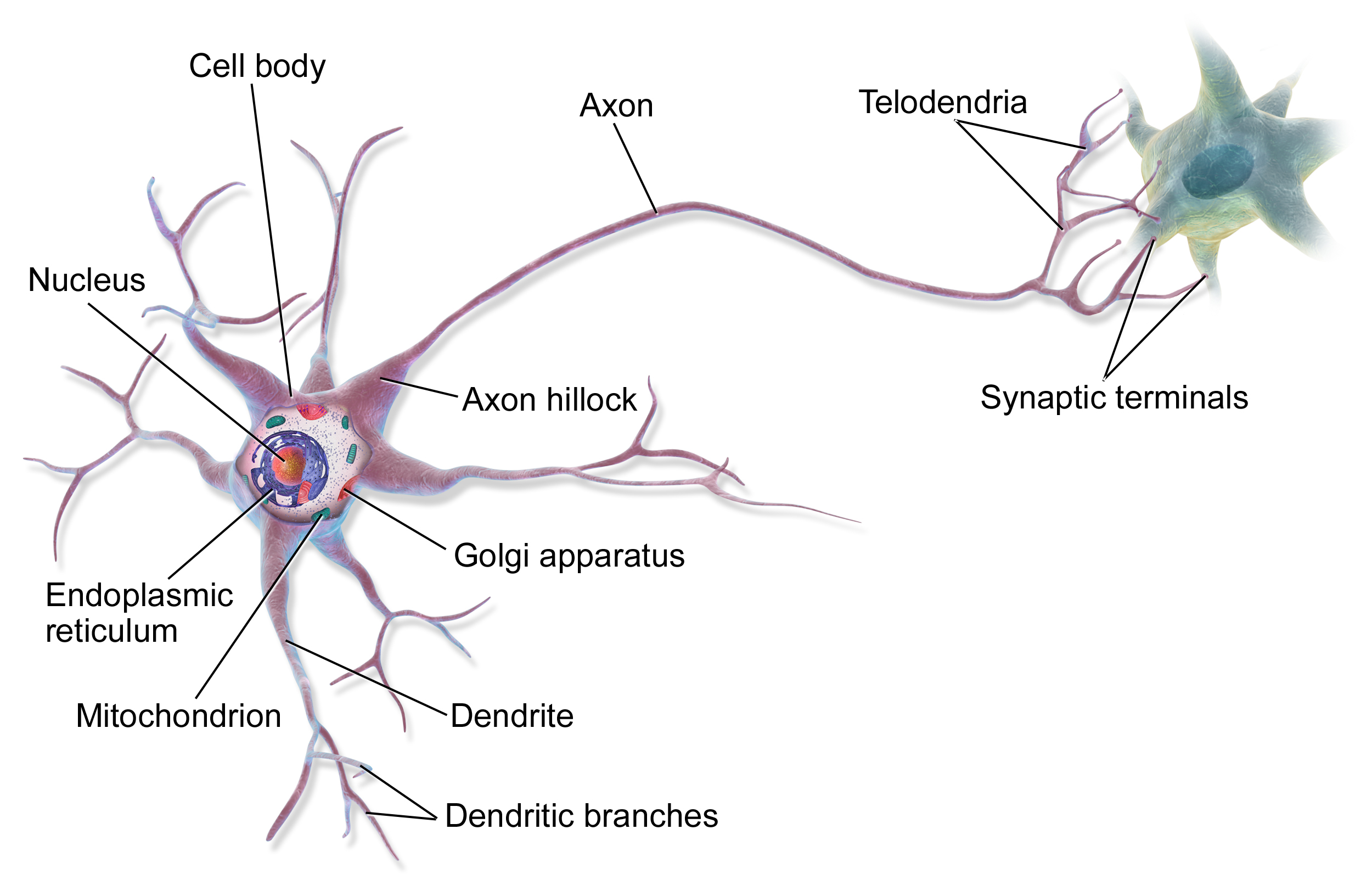
Fig. 1 Our brains are composed of simple processing units, called neurons. Neurons receive signals (information) from other neurons, process those signals and produce an output signal to other neurons. [Drawing by BruceBlaus - Own work, CC BY 3.0, https://commons.wikimedia.org/w/index.php?curid=28761830]

The branches of an axon, each carrying the same information, connect to other neurons’ dendrites (Fig. 2). The connection with another neuron is called the synapse. What travels through the synapse are called neurotransmitters. Without going into details, one can simplify the action of neurotransmitters as messengers that cause an excitation or inhibition on the receiving end. In other words, the neurotransmitters, through a chemical process along the axon, are released into the synapse as the ‘output’ of the neuron, they ‘interact’ with the dendrite (i.e. the ‘input’) of another neuron and potentially lead to an excitation or an inhibition.

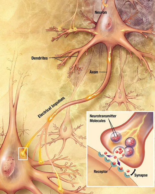
Fig. 2 Neurons ‘communicate’ with each other by transmitting neurotransmitters via synapses. [Drawing by user:Looie496 created file, US National Institutes of Health, National Institute on Aging created original - http://www.nia.nih.gov/alzheimers/publication/alzheimers-disease-unraveling-mystery/preface, Public Domain, https://commons.wikimedia.org/w/index.php?curid=8882110]

Interestingly enough, the synapse is like a valve, which reduces the neurotransmitters’ flow. We will come to this in a second. Now, all the neurotransmitters flown in through the input channels (dendrites) have an accumulative effect on the (receiving) neuron. The neuron emits a neurotransmitter burst through its axon. This emission is not a ‘what-comes-in-goes-out’ type. It is more like the curve in Fig. 3.

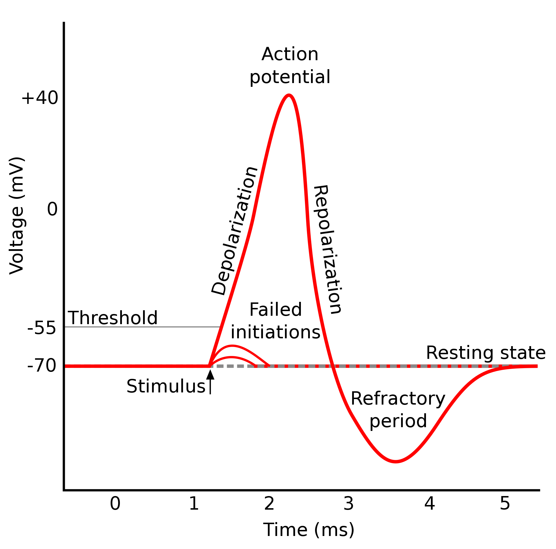
Fig. 3 When a neuron receives ‘sufficient’ amount of signals, i.e. stimulated, it emits neurotransmitters on its axon, i.e. it fires. [Plot by Original by en:User:Chris 73, updated by en:User:Diberri, converted to SVG by tiZom - Own work, CC BY-SA 3.0, https://commons.wikimedia.org/w/index.php?curid=2241513]

The throughput of the synapse is something that may vary with time. Most synapses have the ability to ease the flow over time if the neurotransmitter amount that entered the synapse was constantly high. High activity widens the synaptic connection. The reverse also happens: Less activity over time narrows the synaptic connection.

Some neurons are specialized in creating neurotransmitter emission under certain physical effects. Retina neurons, for example, create neurotransmitters if light falls on them. Some, on the other hand, create physical effects, like creating an electric potential that will activate a muscle cell. These specialized neurons feed the huge neural net, the brain, with inputs and receive outputs from it.

The human brain, containing about \(10^{11}\) such neurons with each neuron being connected to 1000-5000 other neurons by the mechanism explained above, is a very unique computing ‘machine’ that inspires computational sciences.

A short video on synaptic communication between neurons

# Hide code

Video 1. A detailed illustration of how neurotransmitters are transmitted at synapses. [Video from https://www.youtube.com/watch?v=WhowH0kb7n0]

The brain never stops processing information and the functioning of each neuron is only based on signals (the neurotransmitters) it receives through its connections (dendrites). There is no common synchronization timing device for the computation: i.e. each neuron behaves on its own and functions in parallel.

An interesting phenomenon of the brain is that the information and the processing are distributed. Thanks to this feature, when a couple of neurons die (which actually happens each day) no information is lost completely.

On the contrary to the brain, which uses varying amounts of chemicals (neurotransmitters), the microprocessor based computational machinery uses the existence and absence of an electric potential. The information is stored very locally. The microprocessor consists of subunits but they are extremely specialized in function and far less in number compared to \(10^{11}\) all alike neurons. In the brain, changes take place at a pace of 50 Hz maximum, whereas this pace is \(10^{9}\) Hz in a microprocessor.

In Chapter 1, we will take a closer look at the microprocessor machinery which is used by today’s computers. Just to make a note, there are man-made computing architectures other than the microprocessor. A few to mention would be the ‘analog computer’, the ‘quantum computer’ and the ‘connection machine’.

iv. What is a ‘computer’?

As you have already noticed, the word ‘computer’ is used in more than one context.

1. The broader context: Any physical entity that can do ‘computation’.

2. The most common context: An electronic device that has a ‘microprocessor’ in it.

From now on, ‘computer’ will refer to the second meaning, namely a device that has a ‘microprocessor’.

A computer…

• is based on binary (0/1) representations such that all inputs are converted to 0s and 1s and all outputs are converted from 0/1 representations to a desired form, mostly a human-readable one. The processing takes places on 0s and 1s, where 0 has the meaning of ‘no electric potential’ (no voltage, no signal) and 1 has the meaning of ’some fixed electric potential (usually 5 Volts, a signal).

• consists of two clearly distinct entities: The Central Processing Unit (CPU), also known as the microprocessor (𝜇P), and a Memory. In addition to these, the computer is connected to or incorporates other electronic units, mainly for input-output, known as ‘peripherals’.

• performs a ‘task’ by executing a sequence of instructions, called a ‘program’.

• is deterministic. That means if a ‘task’ is performed under the same conditions, it will produce always the same result. It is possible to include randomization in this process only by making use of a peripheral that provides electronically random inputs.

v. What is programming?

The CPU (the microprocessor - 𝜇P) is able to perform several types of actions:

• Arithmetic operations on binary numbers that represent (encode) integers or decimal numbers with fractional part.

• Operations on binary representations (like shifting of digits to the left or right; inverting 0s and 1s).

• Transferring to/from memory.

• Comparing numbers (e.g. whether a number \(n_1\) larger than \(n_2\)) and performing alternative actions based on such comparisons.

• Communicating with the peripherals.

• Alternating the course of the actions.

Each such unit action is recognized by the CPU as an instruction. In more technically terms, tasks are solved by a CPU by executing a sequence of instructions. Such sequences of instructions are called machine codes. Constructing machine codes for a CPU is called ‘machine code programming’.

But, programming has a broader meaning:

a series of steps to be carried out or goals to be accomplished.

And, as far as computer programming is concerned, we would certainly like these steps to be expressed in a more natural (more human readable) manner, compared to binary machine codes. Thankfully, there exist ‘machine code programs’ that read-in such ‘more natural’ programs and convert them into ‘machine code programs’ or immediately carry out those ‘naturally expressed’ steps.

Python is such a ‘more natural way’ of expressing programming steps.