4. Dive into Python Colab

Open the notebook in Colab

(C) Copyright Notice: This chapter is part of the book available athttps://pp4e-book.github.io/and copying, distributing, modifying it requires explicit permission from the authors. See the book page for details:https://pp4e-book.github.io/

After having covered some background on how a computer works, how we solve problems with computers and how we can represent data in binary, we are ready to interact with Python and to learn representing data and performing actions in Python.

The Python interpreter that we introduced in Chapter 2 waits for our computational demands if not executing something already. Those demands that describe an algorithm have to be expressed in Python as a sequence of ‘actions’ where each action can serve two broad purposes:

• Creating or modifying data: These actions take in data, perform sequential, conditional or repetitive execution on the data, and produce other data. Computations that form the bases for our solutions are going to be these kinds of actions.

• Interacting with the environment: Our solutions will usually involve interacting with the user or the peripherals of the computer to take in (input) data or take out (output) data.

Irrespective of its purpose, an action can be of two types:

• Expression: An expression (e.g. 3 + 4 * 5) specifies a calculation, which, when evaluated (performed), yields some data as a result. An expression can consist of:

  • basic data (integer, floating point, boolean etc.) or container data (e.g. string, list, set etc.).

  • expressions involving operations among data and other expressions.

  • functions acting on expressions.

• Statement: Unlike an expression, a statement does not return data as a result and can be either basic or compound:

  • Basic statement: A basic statement can be e.g. for storing the result of an expression in a memory location (an assignment statement for further use (in following actions), deleting an item from a collection of data etc. Each statement has its special syntax that generally involves a special keyword.

  • Compound statement: Compound statements are composed of other statements and executing the compound statement means executing the statements in the compound.

Naming and Printing Data

For better illustrations and examples, we will use two concepts in the first part of the chapter before they are introduced. Let us briefly describe them and leave the coverage of the details to their individual sections:

• Variables: In programming languages, we can give a name to data and use that name to access it, e.g.:

  >>> a = 3
  >>> 10 + a
  13
  

  We call such names variables and the action a = 3 is called an assignment. We defer a more detailed coverage until Section 4.4.

• Printing data: Python provides the print() function to display data items on screen:

  print(item1, item2, ..., itemN)
  

  For example:

  >>> print('Python', 'is', 'so', 'fun')
  Python is so fun
  

4.1. Basic Data

Let us remember what basic data types we had:

• Numbers

  • Integers

  • Floating points

  • Complex numbers

• Booleans

Python is a language in which all arithmetic operations among the same type of numbers are provided very much as expected from our math knowledge. Furthermore, mixed type operations (e.g. subtracting a floating point number form an integer) are also defined.

In programming, being able to ask questions about data is of vital importance. The atomic structures for asking questions are the comparison operations (e.g. “is a value equal to another value”, or “is a value greater than another value”, etc.). Operators that serve these purposes do exist in Python and provide resulting values that are True or False (Booleans). It is also possible to combine such questions under logical operations. The and, or and not operators stand for conjunction, disjunction and negation, correspondingly. Needless to say, these operators also return Boolean values.

4.1.1. Numbers in Python

Python provides the following representations for numbers (the following is an essential reminder from the previous chapter):

• Integers: You can use integers as you are used to from your math classes. Interestingly Python adopts a seamless internal representation so that integers can effectively have any number of digits. The internal mechanism of Python switches from the CPU-imposed fixed-size integers to some elaborated big-integer representation silently when needed. You do not have to worry about it. Furthermore, bear in mind that “73.” is not an integer in Python. It is a floating point number (73.0). An integer cannot have a decimal point as part of it.

• Floating point numbers (float in short): In Python, numbers which have decimal point are taken and represented as floating point numbers. For example, 1.45, 0.26, and -99.0 are float but 102 and -8 are not. We can also use the scientific notation (\(a \times 10^b\)) to write floating point numbers. For example, float 0.0000000436 can be written in scientific notation as \(4.36 \times 10^{-8}\) and in Python as 4.36E-8 or 4.36e-8.

• Complex numbers: In Python, complex numbers can be created by using j after a floating point number (or integer) to denote the imaginary part: e.g. 1.5-2.6j for the complex number \((1.5-2.6i)\). The j symbol (or \(i\)) represents \(\sqrt{-1}\). There are other ways to create complex numbers, but this is the most natural way, considering your previous knowledge from highschool.

More on Integers and Floating Point Numbers

Python provides int data type for integers and float data type for floating point numbers. You can easily play around with int and float numbers and check their type as follows:

>>> 3+4
7
>>> type(3+4)
<class 'int'>
>>> type(4.1+3.4)
<class 'float'>

where <class 'int'> indicates type int.

In Python version 3, integers do not have fixed-size representation and their size is only limited by your available memory. In Python version 2, there were two integer types: int, which used the fixed length representation supported by the CPU, and long type, which was unbounded. Since this book is based on Python version 3, we will assume that int refers to an unbounded representation.

As for the float type, Python uses the 64-bit IEEE754 standard, which allows representing numbers in the range [2.2250738585072014E-308, 1.7976931348623157E+308].

Useful Operations:

The following operations can be useful while working with numbers:

• abs(<Number>): Takes the absolute value of the number.

• pow(<Number1>, <Number2>): Takes the power of <Number1>, i.e. \(\textrm{<Number1>}^{\textrm{<Number2>}}\)

• round(<FloatNumber>): Rounds the floating point number to the closest integer.

• Functions from the math library: sqrt(), sin(), cos(), log(), etc (see the Python documentation for a full list). This requires importing from the built-in math library first as follows:

  >>> from math import *
  >>> sqrt(10)
  3.1622776601683795
  >>> log10(3.1622776601683795)
  0.5
  

4.1.2. Boolean Values

Python provides the bool data type which allows only two values: True and False. For example:

>>> type(True)
<class 'bool'>
>>> 3 < 4
True
>>> type(3 < 4)
<class 'bool'>

Also due to decades of programming experience, Python converts several instances of other data types to some certain boolean values, if used in place of a boolean value. For example,

• 0 (the integer zero)

• 0.0 (the floating point zero)

• "" (the empty string)

• [] (the empty list)

• {} (the empty dictionary or set)

are interpreted as False. All other values of similar kinds are interpreted as True.

Useful Operations:

With boolean values, we can use not (negation or inverse), and and or operations:

>>> True and False
False
>>> 3 > 4 or 4 < 3
False
>>> not(3 > 4)
True

and returns a True value only if both of its operands are True, otherwise it returns False. or returns True if any or both of its operands are True. The following table gives result of the boolean operations for the given operand pair:

a	b	a and b	a or b
True	True	True	True
True	False	False	True
False	True	False	True
False	False	False	False

4.2. Container data (str, tuple, list, dict, set)

Up to this point we have seen the basic data types. They are certainly needed for computation but many world problems for which we seek computerized solutions need more elaborate data. Just to mention a few:

• Vectors

• Matrices

• Ordered and unordered sets

• Graphs

• Trees

Vectors and matrices are used in almost all simulations/problems of the physical world; sets are used to keep any property information as well as orders of items, equivalences; graphs are necessary for many spatial problems; trees are vital to representing hierarchical relational structures, action logics, organizing data for a quick search.

Python provides five container types for these:

1. String (``str``): A string can hold a sequence of characters or only a single character. A string cannot be modified after creation.

2. List (``list``): A list can hold ordered sets of all data types in Python (including another list). A list’s elements can be modified after creation.

3. Tuple (``tuple``): The tuple type is very similar to the list type but the elements cannot be modified after creation (similar to strings).

4. Dictionary (``dict``): A very very efficient method to form a mapping from a set of numbers, booleans, strings and tuples to any set of data in Python. Dictionaries are easily modifiable and extendable. Querying the mapping of an element to the ‘target’ data is performed in almost constant time (regardless of how many elements the dictionary has). In Computer Science terms, it is a hash table.

5. Set (``set``): The set type is equivalent to sets in mathematics. The element order is undefined. (We deemphasize the use ofset).

The first three, namely String, List and Tuple are called sequential containers. They consist of consecutive elements indexed by integer values starting at 0. Dictionary is not sequential, element indexes are arbitrary. For simplicity we will abbreviate sequential containers as s-containers.

All these containers have external representations which are used in inputting and outputting them (with all their content). Below we will walk through some examples to explain them.

Mutability vs. Immutability

Some container types are created ‘frozen’. After creating them you can wholly destroy them but you cannot change or delete their individual elements. This is called immutability. Strings and tuples are immutable whereas lists, dictionaries and sets are mutable. With a mutable container, adding new elements and changing or deleting existing ones is possible.

4.2.1. Accessing elements in sequential containers

All containers except set reveal their individual elements by an indexing mechanism with brackets:

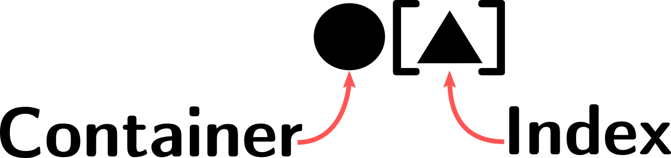
Fig. 4.2.1 How elements of a container are accessed

For the s-containers, the index is an ordinal number where counting starts with zero. For dictionaries, the index is a Python data item from the source (domain) set. A negative index (usable only on s-containers) has a meaning that the (counting) value is relative to the end. A negative index can be converted to a positive index by adding to the negative value the length of the container. It is nothing but index obtained by adding the length of the container.

Below we have an s-container that has a length of \((n+1)\)

(careful: indexing started at 0!):

(4.2.1)\[\begin{split}\begin{array}[t]{|c|c|c} \hline \;\Box_0 & \;\Box_1 & \\ \hline \end{array} \cdots \begin{array}[t]{c|c|c|} \hline & \;\Box_{n-1} & \; \Box_n\; \\ \hline \end{array}\\ \begin{array}[t]{ccc} \mathtt{[0]}& \; \mathtt{[1]} & \\ \end{array} \;\cdots \begin{array}[t]{ccc} & \;\mathtt{[}{\scriptsize n-1}\mathtt{]} & \; \mathtt{[}{\scriptsize n}\mathtt{]} \\ \end{array} \\ \!\!\!\! \begin{array}[t]{ccc} \mathtt{[}{\scriptsize -(n+1)}\mathtt{]} & \!\!\!\!\!\mathtt{[}{\scriptsize -n}\mathtt{]}\! & \\ \end{array} \; \cdots \;\; \begin{array}[t]{ccc} & \mathtt{[-2]} & \mathtt{[-1]} \\ \end{array}\end{split}\]

As you surely have observed, when you add \((n+1)\) to the negative index you obtain the positive one.

Slicing

s-containers provide a rich mechanism, called slicing, that allows accessing multiple elements at once. Thanks to this mechanism, you can define a start and end index and obtain the portion that lies in between (Fig. 4.2.2):

• The element at the start index is the first to be accessed.

• The end index is where accessing stops (the element at the end index is not accessed – i.e. the end index is not inclusive).

• It is also possible to optionally define an increment (jump amount) between indexes. After the element at \(\mathtt{[}start\mathtt{]}\) is accessed first, \(\mathtt{[}start+increment\mathtt{]}\) is accessed next. This goes on until the accessed position is equal or greater than the end index. For negative indexing, a negative increment has to work from the bigger index towards the lesser, so \((start\ index>end\ index)\) is expected.

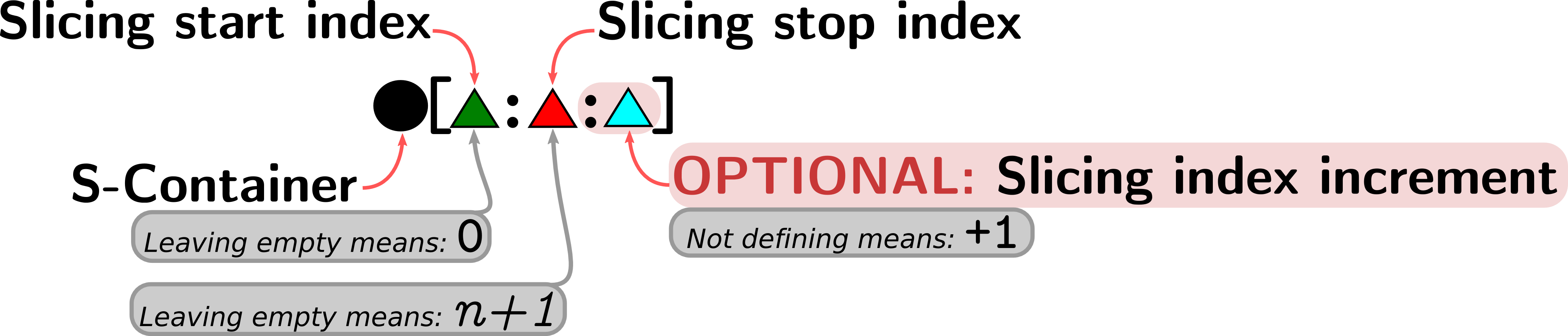
Fig. 4.2.2 Accessing multiple elements of an s-container is possible via the slicing mechanism, which specifies a starting index, an ending index and an index increment between elements.

Below, with the introduction of strings, we will have extensive examples on slicing.

If the s-container is immutable (e.g. string and tuple containers) then slicing creates a copy of the sliced data. Otherwise, i.e. if the s-container is mutable (i.e. the ‘list’ container) then slicing provides direct access to the original elements and therefore, they can be updated, which updates the original s-container.

4.2.2. Useful operations common to containers

The following operations are common to all or a subset of containers:

1- Number of elements:

For all containers len() is a built-in function that returns the count of elements in the container that is given as argument to it, e.g.:

>>> len("Five")
4

2- Concatenation:

String, tuple and list data types can be combined using ‘+’ operation:

<Container1> + <Container2>

where the containers need to be of the same type. For example:

>>> "Hell" + "o"
'Hello'

3- Repetition: String, tuple and list data types can be repeated using “*” operation:

<Container1> * <Number>

where the container is copied ‘’ many times. For example:

>>> "Yes No " * 3
'Yes No Yes No Yes No '

4- Membership: All containers can be checked for whether they contain a certain item as an element using in and not in operations:

<item> in <Container>

or

<item> not in <Container>

Of course, the result is either True or False. For dictionaries in tests if the domain set contains the element, for others it simply tests if element is a member.

4.2.3. String

As was explained in the previous chapter, a string is used to hold a sequence of characters. Actually, it is a container where each element is a character. However, Python does not have a special representation for a single character. Characters are represented externally as strings containing a single character only.

Writing strings in Python

In Python a string is denoted by enclosing the character sequence between a pair of quotes (') or double quotes ("). A string surrounded with triple double quotes (""" \(\ldots\) """) allows you to have any combination of quotes and line breaks within a sequence, and Python will still view it as a single entity.

Here are some examples:

• "Hello World!"

• 'Hello World!'

• 'He said: "Hello World!" and walked towards the house.'

• "A"

• """ Andrew said: "Come here, doggy". The dog barked in reply: 'woof' """

The backslash (\) is a special character in Python strings, also known as the escape character. It is used in representing certain, the so called, unprintable characters: (\t) is a tab, (\n) is a newline, and (\r) is a carriage return. Table 4.2.1 provides the full list.

Table 4.2.1 The list of escape characters in Python.

Escape Sequence	Meaning
\\	Backslash (\)
\'	Single quote (')
\"	Double quote (")
\a	ASCII Bell (BEL)
\b	ASCII Backspace (BS)
\f	ASCII Formfeed (FF)
\n	ASCII Linefeed (LF)
\r	ASCII Carriage Return (CR)
\t	ASCII Horizontal Tab (TAB)
\v	ASCII Vertical Tab (VT)
\ooo	ASCII character with octal value ooo
\xhh	ASCII character with hex value hh
\uhhhh	UNICODE character with hex value hhhh

Conversely, prefixing a special character with (\) turns it into an ordinary character. This is called escaping. For example, (\') is the single quote character. 'It\'s raining' therefore is a valid string and equivalent to "It's raining". Likewise, (") can be escaped: "\"hello\"" is a string that begins and ends with the literal double quote character. Finally, (\) can be used to escape itself: (\\) is the literal backslash character. For '\onnn', nnn is a number in base 8, for '\xnn' nn is a number in base 16 (including letters from A to F as digits for values 10 to 15).

In Python v3, all strings use the Unicode representation where all international symbols are possible, e.g.:

>>> a = "Fıstıkçı şahap"
>>> a
'Fıstıkçı şahap'

Examples with strings

Let us look at some examples to see what strings are in Python and what we can do with them:

>>> "This is a string"
"This is a string"
>>> "This is a string"[0]
'T'
>>> s = "This is a string"
>>> print(s[0])
T
>>> print(s[0],s[1],s[8],s[14],s[15])
T h a n g

Since strings are immutable an attempt to change a character in a string will badly fail:

>>> s = "This is a string"
>>> print(s)
This is a string
>>> s[2] = "u"
Traceback (most recent call last):
  File "<stdin>", line 1, in <module>
TypeError: 'str' object does not support item assignment

Bottom line: You cannot change a character in a created string.

Let us go through a sequence of examples. We encourage you to run the following examples in the Colab version of this chapter. Feel free to change the text and rerun the examples.

# Hide code

my_beautiful_string  = "The quick brown fox jumps over the lazy dog"
print("THE STRING:", my_beautiful_string, len(my_beautiful_string), "CHARACTERS")

THE STRING: The quick brown fox jumps over the lazy dog 43 CHARACTERS

my_beautiful_string[0]

'T'

my_beautiful_string[4]

'q'

my_beautiful_string[0:4]

'The '

my_beautiful_string[:4]

'The '

my_beautiful_string[4:]

'quick brown fox jumps over the lazy dog'

my_beautiful_string[10:15]

'brown'

my_beautiful_string[:-5]

'The quick brown fox jumps over the laz'

my_beautiful_string[-8:-5]

'laz'

my_beautiful_string[:]

'The quick brown fox jumps over the lazy dog'

my_beautiful_string[::-1]

'god yzal eht revo spmuj xof nworb kciuq ehT'

my_beautiful_string[-6:-9:-1]

'zal'

my_beautiful_string[0:15:2]

'Teqikbon'

Strings are used to represent non-mathematical textual information. Common places where strings are used are:

• Textual communation in natural language with the user of the program.

• Understandable labeling of parts of data: City names, names of individuals, addresses, tags, labels.

• Denotation needs of human-to-human interactions.

Useful operations with strings:

• String creation: In addition to using quotes for string creation, the str() function can be used to create a string from its argument, e.g.:

  >>> str(4)
  '4'
  >>> str(4.578)
  '4.578'
  

• Concatenation, repetition and membership:

  >>> 'Programming' + ' ' + 'with ' + 'Python is' + ' fun!'
  'Programming with Python is fun!'
  >>> 'really fun ' * 10
  'really fun really fun really fun really fun really fun really fun really fun really fun really fun really fun '
  >>> 'fun' in 'Python'
  False
  >>> 'on' in 'Python'
  True
  

• Evaluate a string: If you have a string that is an expression describing a computation, you can use the eval() function to evaluate the computation and get the result, e.g.:

  >>> s = '3 + 4'
  >>> eval(s)
  7
  

Deletion and Insertion from/to strings

Since strings are immutable, this is not possible. The only way is to create a new string, making use of slicing and concatenation operation (using +), then replacing the new created string in same place of the former one. For example:

>>> a = 'Python'
>>> a[0] = 'S'
Traceback (most recent call last):
  File "<stdin>", line 1, in <module>
TypeError: 'str' object does not support item assignment
>>> b = 'S' + a[1:]
>>> b
'Sython'

4.2.4. List and tuple

Both list and tuple data types have a very similar structure on the surface: They are sequential containers that can contain any other data type (including other tuples or lists) as elements. The only difference concerning the programmer is that tuples are immutable whereas lists are mutable. As previously said, being immutable means that, after being created, it is not possible to change, delete or insert any element in a tuple.

Lists are created by enclosing elements into a pair of brackets and separating them with commas, e.g. ["this", "is", "a", "list"]. Tuples are created by enclosing elements into a pair of parentheses, e.g. ("this", "is", "a", "tuple"). There is no restriction on the elements: They can be any data (basic or container).

Let us look at some examples for lists:

• [9,3,1,-1,6]

• []

• [2020]

• [3.1415, 2.718281828]

• [["pi,3.1415"], ["e",2.718281828], 1.41421356]

• the' 'quick','brown','fox','jumped','over','the','lazy','dog

• [10, [5, [3, [[30, [[30, [], []]], []]], []], [8, [], []]], [30, [], []]]

• [[1,-1,0],[2,-3.5,1.1]]

and some examples for tuples:

• ('north','east','south','west')

• ()

• ('only',)

• ('A',65,"1000001","0x41")

• ("abx",[1.32,-5.12],-0.11)

Of course, tuples can become list members as well, or vice versa:

• [("ahmet","akhunlar",("deceased", 1991)), ("huri","huriyegil","not born")]

• (["ahmet","akhunlar",("deceased", 1991)], ["huri","huriyegil","not born"])

Programmers generally prefer using lists over tuples since they allow changing elements, which is often a useful facility in many problems.

Lists (and tuples) are used whenever there is a need for an ordered set. Here are a few usecases for lists and tuples:

• Vectors.

• Matrices.

• Graphs.

• Board game states.

• Student records, address book, any inventory.

Useful operations with lists and tuples

1- Deletion from lists

As far as deletion is concerned, you can use two methods:

• Assigning an empty list to the slice that is going to be removed:

>>> L = [111,222,333,444,555,666]
>>> L[1:5] = []
>>> print(L)
[111, 666]

• Using the del statement on the slice that is going to be removed:

>>> L = [111,222,333,444,555,666]
>>> del L[1:5]
>>> print(L)
[111, 666]

2- Insertion into lists

For insertion, you can use three methods:

• Using assignment with a degenerate use of slicing:

>>> L = [111,222,333,444,555,666]
>>> L[2:2] = [888,999]
>>> print(L)
[111, 222, 888, 999, 333, 444, 555, 666]

• The second method can insert only one element at a time, and requires object-oriented features, which will be covered in Chapter 7.

>>> L = [111,222,333,444,555,666]
>>> L.insert(2, 999)
>>> print(L)
[111, 222, 999, 333, 444, 555, 666]

where the insert function takes two parameters: The first parameter is the index where the item will be inserted and the second parameter is the item to be inserted.

• The third methods uses the append() method to insert an element only to the end or extend() to append more than one element to the end:

>>> L = [111,222,333,444,555]
>>> L.append(666)
>>> print(L)
[111, 222, 333, 444, 555, 666]
>>> L.extend([777, 888])
[111, 222, 333, 444, 555, 666, 777, 888]

3- Data creation with ``tuple()`` and ``list()`` functions: Similar to other data types, tuple and list data types provide two functions for creating data from other data types.

4- Concatenation and repetition with lists and tuples: Similar to strings, + and * can be used respectively to concatenate two tuples/lists and to repeat a tuple/list many times.

5- Membership: Similar to strings, in and not in operations can be used to check whether a tuple/list contains an element.

Here is an example that illustrates the last three items:

>>> a = ([3] + [5])*4
>>> a.append([3, 5])
>>> print(a)
[3, 5, 3, 5, 3, 5, 3, 5, [3, 5]]
>>> a.extend([3, 5])
>>> print(a)
[3, 5, 3, 5, 3, 5, 3, 5, [3, 5], 3, 5]
>>> b = tuple(a)
>>> print(b)
(3, 5, 3, 5, 3, 5, 3, 5, [3, 5], 3, 5)
>>> [3, 5] not in b
False
>>> [5, 3] not in b
True             #  test for single element, not subsequence

As you have recognized, the examples with some containers included two types of constructs which were not covered yet: One is the use of ‘functions’ on containers, e.g. the use of len(). Due to your high school background, this is certainly easy to understand. The second construct is something new. It appears that we can use some functions suffixed by a dot to a container (e.g. the append and insert usages in the examples above). This construct is an internal function call of data structure called object. Containers are actually objects and in addition to their data containment property, they also have some defined action associations. These actions are named as member functions, and called (applied) on that object (in our case -the container-) by means of this dot notation:

(4.2.2)\[{\Huge\bullet}{\large.}{\Large f(\Box)}\quad\mbox{has the conceptual meaning of}\quad{\Large f({\Huge\bullet},\Box)}\]

(Don’t try this explicitly, it will not work. The equivalence is just ‘conceptual’: meaning the function receives the object internally, as a ‘hidden’ argument). All these will be covered in details in Chapter 7. Till then, for sake of completeness, from time to time we will referring to this notation. Till then simply interpret it based on the equivalence depicted above.

Example: Matrices as Nested Lists

In many real-world problems, we often end up with a set of values that share certain semantics or functionality, and benefit from representing them in a regular grid structure that we call matrix:

(4.2.3)\[\begin{split}A = \begin{pmatrix} a_{11} & a_{12} & ... & a_{1n} \\ a_{21} & a_{22} & ... & a_{2n} \\ \vdots & \ddots & & \vdots & \\ a_{m1} & a_{m2} & ... & a_{mn} \end{pmatrix},\end{split}\]

which has \(n\) columns and \(m\) rows, and we generally shorten this as \(m\times n\) and say that matrix \(A\) has size \(m\times n\). The following set of equations describe relations among a set of variables and called system of equations:

(4.2.4)\[\begin{split}\begin{array}{ccc} 3x + 4y + z & = & 4,\\ -3x + 3y + 5 & = & 3,\\ x + y + z & = & 0,\\ \end{array}\end{split}\]

which can be represented with matrices as:

(4.2.5)\[\begin{split}\begin{pmatrix} 3 & 4 & 1 \\ -3 & 3 & 5 \\ 1 & 1 & 1 \end{pmatrix} \begin{pmatrix} x \\ y \\ z \end{pmatrix} = \begin{pmatrix} 4 \\ 3 \\ 0 \end{pmatrix} ,\end{split}\]

which defines the same problems in terms of matrices and matrix multiplication. It is okay if you are not familiar with matrix multiplication – we will briefly explain it and use it as an example in the next chapter.

Writing a problem in a matrix form like we did above allows us to group the related aspects of the problem together and focus on these groups for solving a problem. In our example, we grouped coefficients in a matrix and this allows us to analyze and manipulate the coefficients matrix to check whether for this system of equations there is a solution, whether the solution is unique or what the solution is. All these are questions that are studied in Linear Algebra and beyond the scope of our book.

Now let us see how we can represent matrices in Python. A very straightforward approach that would also allow changing elements of the matrix later on is to use lists in a nested form, as follows:

>>> A = [[3, 4, 1],
... [-3, 3, 5],
... [1, 1, 1]]
>>> A
[[3, 4, 1], [-3, 3, 5], [1, 1, 1]]

where each row is represented as a list and a member of the outer list. This would allow us to access entries like this:

>>> A[1]
[-3, 3, 5]
>>> A[1][0]
-3

Although we can represent matrices like this, there are very advanced libraries that make representing and working with matrices more practical, as we will see in Chapter 10. For an extended coverage on matrices and matrix operations, we refer to Matrix algebra for beginners (by Jeremy Gunawardena) or Chapter 2.2 of “Mathematics for Machine Learning” (by Marc Peter Deisenroth, A. Aldo Faisal and Cheng Soon Ong).

4.2.5. Dictionary

Dictionary is a container data type where accessing items can be performed with indexes that are not numerical; in fact, in dictionaries, indexes are called keys. A list, tuple, or string data type stores a certain element at each numerical index (key). Similarly, a dictionary stores an element (value) for each key. In other words, a dictionary is just a mapping from keys to values (Fig. 4.2.3).

The keys can be only immutable data types, i.e., numbers, strings, or tuples (with only immutable elements) – some other immutable types that we do not cover in the book are also possible. Since lists and dictionaries are mutable, they cannot be used for keys for indexing. As for values, there is no limitation on the data type.

A dictionary is a discrete mapping from a set of Python elements to another set of Python elements. Itself, as well as its individual elements, are mutable (you can replace them). Moreover, it is possible to add and remove items from the mapping.

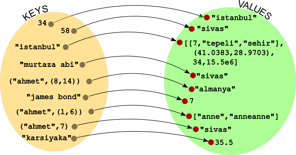
Fig. 4.2.3 A dictionary provides a mapping from keys to values.

A dictionary is represented as key-value pairs, each separated by a column sign (:) and all enclosed in a pair of curly braces. The dictionary in Fig. 4.2.3 would be denoted as:

{34:"istanbul",
 58:"sivas",
 "istanbul":[[7,"tepeli","sehir"],(41.0383,28.9703),34,15.5e6],
 "murtaza abi":"sivas",
 ("ahmet",(8,14)):"almanya","james bond":7,
 ("ahmet",(1,6)):["anne","anneanne"],
 ("ahmet",7):"sivas",
 "karsiyaka":35.5}

Similar to other containers, we usually store containers under a variable. Let us assume the dictionary above was assigned to a variable with the name conno and look at some examples:

conno = {34:"istanbul", 58:"sivas", "istanbul":[[7,"tepeli","sehir"],(41.0383,28.9703),34,15.5e6], "murtaza abi":"sivas", ("ahmet",(8,14)):"almanya","james bond":7,  ("ahmet",(1,6)):["anne","anneanne"], ("ahmet",7):"sivas",   "karsiyaka":35.5}
print(conno["murtaza abi"])
print(conno["istanbul"])

sivas
[[7, 'tepeli', 'sehir'], (41.0383, 28.9703), 34, 15500000.0]

Let us ask for something that does not exist in the dictionary:

>>> print(conno["ankara"])
KeyError: 'ankara'

Ups, that was bad. Though we have a decent method to test for the existence of a key in a dictionary, namely the use of in:

print("ankara" in conno)

False

It is also possible to remove/insert mappings from/to a dictionary:

print("conno has this many keys:", len(conno))
conno["ankara"] = ["baskent", "anitkabir", 6]
print("conno has this many keys now:", len(conno))
print(conno["ankara"])
print(conno["murtaza abi"])
del conno["murtaza abi"]
print("murtaza abi" in conno)
print("After murtaza abi is deleted we have this many keys:", len(conno))

conno has this many keys: 9
conno has this many keys now: 10
['baskent', 'anitkabir', 6]
sivas
False
After murtaza abi is deleted we have this many keys: 9

The benefit of using a dictionary is ‘timewise’. The functionality of a dictionary could be attained by using (key, value) tuples inserted into a list. Then, when you need the value of a certain key, you can search one-by-one each (key, value)-tuple element of the list until you find your key in the first position of a tuple element. However, this will consume a time proportional to the length of the list (worst case). On the contrary, in a dictionary, this time is almost constant.

Moreover, a dictionary is more practical to use since it already provides accessing elements in a key-based fashion.

Useful Operations with Dictionaries

Dictionaries support len() and membership (in and not in) operations that we have seen above. You can also use <dictionary>.values() and <dictionary>.keys() to obtain lists of values and keys respectively.

4.2.6. Set

Sets are created by enclosing elements into a pair of curly-braces and separating them with commas. Any immutable data type, namely a number, a string or a tuple, can be an element of a set. Mutable data types (lists, dictionaries) cannot be elements of a set. Being mutable, sets cannot be elements of a sets.

Here is a small example with sets:

a = {1,2,3,4}
b = {4,3,4,1,2,1,1,1}
print (a == b)
a.add(9)
a.remove(1)
print(a)

True
{2, 3, 4, 9}

The most functionalities of sets can be undertaken by lists. Furthermore, lists do not possess the restrictions sets do. On the other hand, especially membership tests are much faster with sets, since member repetition is avoided.

Frozenset

Python provides an immutable version of the set type, called frozenset. A frozenset can be constructed using the frozenset() function as follows:

>>> s = frozenset({1, 2, 3})
>>> print(s)
frozenset({1, 2, 3})

Being immutable, frozensets can be a member of a set or a frozenset.

Useful Operations with Sets

Apart from the common container operations (len(), in and not in), sets and frozensets support the following operators:

• S1 <= S2: True if S1 is a subset of S2.

• S1 >= S2: True if S1 is a superset of S2.

• S1 | S2: Union of the sets (equivalent to S1.union(S2)).

• S1 & S2: Intersection of the sets (equivalent to S1.intersection(S2)).

• S1 - S2: Set difference (equivalent to S1.difference(S2)).

The following are only applicable with sets (and not with forezensets) as they require a mutable container:

• S.add(element): Add a new element to the set.

• S.remove(element): Remove element from the set.

• S.pop(): Remove an arbitrary element from the set.

4.3. Expressions

Expressions such as 3 + 4 describe calculation of an operation among data. When an expression is evaluated, the operations in the expression are applied on the data specified in the expression and a resulting value is provided.

Operations can be graphically illustrated as follows:

(4.3.1)\[\Box_1 \odot \Box_2\]

where \(\odot\) is called the operator, and \(\Box_1\) and \(\Box_2\) are called operands. This was a binary operator; i.e. it acted on two operands.

We can also have unary operators:

(4.3.2)\[\odot \Box\]

or operators that have more than two operands (see chained comparison operators below).

Before we can cover how such operations are evaluated, let us look at commonly used operations (operators) in Python.

4.3.1. Arithmetic, Logic, Container and Comparison Operations

Python provides the operators in Table 4.3.1 for arithmetic (addition, subtraction, multiplication, division, exponentiation), logic (and, or, not), container (indexing, membership) and comparison (less, less-than, equality, not-equality, greater, greater-than) operations.

Note that operators such as + and * have different meanings on different data types. For numerical data, they mean addition and multiplication whereas for container data, they mean concatenation and repetition.

Table 4.3.1 Arithmetic, Logic, Container and Comparison operators in Python.

Operator	Operation	Result Type
[]	Indexing	Any data type
**	Exponentiation	Numeric
*	Multiplication or Repetition	Numeric or container
/	Division	Numeric (floating point)
//	Integer Division	Numeric (integer)
+	Addition or concatenation	Numeric or container
-	Subtraction	Numeric
<	Less than	Boolean
<=	Less than or equal to	Boolean
>	Greater than	Boolean
>=	Greater than or equal to	Boolean
==	is equal to	Boolean
!=	is not equal to	Boolean
in	is a member	Boolean
not in	is not a member	Boolean
not	logical negation	Boolean
and	logical and	Boolean
or	logical or	Boolean

Below are some illustrations:

S1 = "Four"
S2 = "Five"
B1 = len(S1) < len(S2)
print("B1 is: ", B1)
B2 = S1 != S2
print("B2 is: ", B2)
B3 = B1 or B2
print("B3 is: ", B3)

B1 is:  False
B2 is:  True
B3 is:  True

4.3.2. Exercise

Give one example for each row in Table 4.3.1. Please complete this exercise in the Colab version of the chapter.

4.3.3. Evaluating Expressions

In the previous section, we have seen simple use of operators in an expression. In many cases, we combine several operators for brevity and readability, e.g. 2.3 + 3.4 * 4.5. This expression can be evaluated in two different ways:

• (2.3 + 3.4) * 4.5, which would yield 25.65.

• 2.3 + (3.4 * 4.5), which would yield 17.599999999999998 in Python.

Since the results are very different, it is very important for a programmer to know in which order operators are evaluated when they are combined. There are two rules that govern this:

1. Precedence: Each operator has an associated precedence (priority) based on which we can determine which operator is going to be evaluated first. E.g. multiplication has higher precedence than addition, and therefore, 2.3 + 3.4 * 4.5 would be evaluated as 2.3 + (3.4 * 4.5) in Python.

2. Associativity: If two operators have the same precedence, evaluation order is determined based on associativity. Associativity can be from left to right or from right to left.

For the operators, the complete associativity and precedence information are listed in Table 4.3.2.

Table 4.3.2 Precedence and associativity for the operators in Table 4.3.1.

Operator	Precedence	Associativity
[]		Left-to-right
**		Right-to-left
*, /, //, %		Left-to-right
+, -		Left-to-right
<, <=, >, >=, ==, !=, in, not in		Special
not		Unary
and		Left-to-right (with short-cut)
or		Left-to-right (with short-cut)

Therefore, according to Table 4.3.2, a sophisticated expression such as 2**3**4*5-2//2-1 is equivalent to 2**81*5-1-1 which is equivalent to 12089258196146291747061760-2 which is 12089258196146291747061758.

Below are some notes and explanations regarding expression evaluation:

1. The Special keyword in Table 4.3.2 means some treatment which is common to mathematics but not programming. In that sense Python is unique among commonly used programming languages. If \(\odot_i\) is any boolean comparison operator and \(\Box_j\) is any numerical expression, the sequence of

(4.3.3)\[\Box_1 \odot_{\scriptsize\mathsf 1} \Box_2 \odot_{\scriptsize\mathsf 2} \Box_3 \odot_{\scriptsize\mathsf 3} \Box_4 \cdots \Box_{n-1} \odot_{n-\scriptsize\mathsf 1} \Box_n\]

is interpreted as:

(4.3.4)\[   \Box_1 \odot_{\scriptsize\mathsf 1} \Box_2 \;\;\mathtt{and}\;\;\; \Box_2 \odot_{\scriptsize\mathsf 2} \Box_3\;\;  \mathtt{and} \;\;\; \Box_3 \odot_{\scriptsize\mathsf 3} \Box_4 \;\;\;\cdots \;\;\; \Box_{n-1} \odot_{n-\scriptsize\mathsf 1} \Box_n\]

2. It is always possible to override the precedence by making use of parenthesis. We are familiar with this since our primary school days.

3. If two numeric operands are of the same type, then the result is of that type unless the operator is / (for which the result is always a floating point number). Also comparison operators return bool typed values.

4. If two numeric operands that enter an operation are of different types, then a computation occurs according to the following rules:

• if one operand is integer and the other is floating point: The integer is converted to floating point.

• if one operand is complex: The complex arithmetic is carried out according to the rules of mathematics among the real/imaginary part coefficients (which are either integers or floating points). Each of the two resulting coefficients are separately checked for having zero (.0) fractional part. If so, that one is converted to integer.

22. Except for the two logical operators and and or, all operators have an evaluation scheme which is coined as eager evaluation. Eager evaluation is the strategy where all operands are evaluated first and then the semantics of the operators kicks in, providing the result. Here is an example: Consider mathematical expression of: 0*(2**150-3**95) As a human being, our immediate reaction would be: Anything multiplied with 0 (zero) is 0, therefore we do not have to compute the two huge exponentiations (the second operand). This is taking a short-cut in evaluation and is certainly far from eager evaluation. Eager evaluation would evaluate the internals of the parenthesis, obtain -693647454339354238433323618063349607247325483 and then multiply this with 0 to obtain 0. Yes, Python  would go this ‘less intelligent’ way and do eager evaluation. The logical operators and and or, though, do not adopt eager evaluation. On the contrary, they use short-cuts (this is known as based-on-need evaluation in computer science).

In a conjunctive expression like:

(4.3.5)\[\Box_1 \;\;\mathtt{and}\;\;\; \Box_2  \;\;\mathtt{and}\;\;\; \Box_3 \;\;\mathtt{and}\;\;\; \cdots \;\;\mathtt{and}\;\;\; \Box_n\]

The evaluation proceeds as follows:

Fig. 4.3.1 Logical AND evaluation scheme

  Similarly, a disjunctive expression:

(4.3.6)\[\Box_1 \;\;\mathtt{or}\;\;\; \Box_2  \;\;\mathtt{or}\;\;\; \Box_3 \;\;\mathtt{or}\;\;\; \cdots \;\;\mathtt{or}\;\;\; \Box_n\]

has the following evaluation scheme:

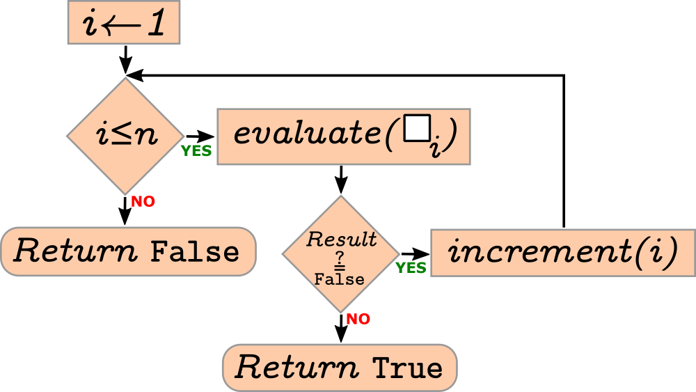
Fig. 4.3.2 Logical OR evaluation scheme

Although high-level languages provide mechanisms for evaluating expressions involving multiple operators, it is not a good programming practice to leave multiple operators without parentheses. A programmer should do his/her best to write code that is readable and understandable by other programmers and that does not include any ambiguity whatsoever. This includes expressions.

4.3.4. Implicit and Explicit Type Conversion

In Python, when you apply a binary operator on items of two different data types, it tries to convert one data to another one if possible. This is called implicit type conversion. For example,

>>> 3+4.5
7.5
>>> 3 + True
4
>>> 3 + False
3

which illustrates that an integer is converted to a float, True is converted to integer 1, and False is converted to integer zero.

Although Python can do such conversions, it is a good programming practice to make these conversions explicit and make the intention clear to the reader. Explicit type conversion, also called as type casting, can be performed using the keyword for the target type as a function. For example:

>>>> 1.1*(7.1+int(2.5*5))
21.01

Not all conversions are possible, of course. Implicit conversions are allowed only for the basic data types as illustrated below:

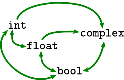
Fig. 4.3.3 Type casting among numeric and Boolean

Type casting can accommodate conversion between a wider spectrum of data types, including containers:

>>> str(34)
'34'
>>> list('34')
['3', '4']

4.4. Basic Statements

Now, let us continue with actions that do not provide (return) us data as a result.

4.4.1. Assignment Statement and Variables

When we perform computation in Python, we either print the result and/or keep the result for further computations that we are going to perform. Variables help us here as named memory positions in which we can store data. You can imagine them as pigeonholes that are able to hold a single data item.

There are two methods to create and store some data into a variable. Here we will mention the overwhelmingly used one, the second is more implicit and will be introduced when we deal with functions.

A variable receives data for storage by the use of the assignment statement. It has the following form:

\(\boxed{\color{red}{Variable}} = \boxed{\color{red}{Expression}}\)

Although the equal sign resembles an operator that is placed between two operands, it is not an operator: Operators return a value, and in Python, the assignment is not an operator and it does not return a value (this can be different in other programming languages).

The action semantics of the assignment statement is simple:

1. The \(\color{red}{Expression}\) is evaluated.

2. If the \(\color{red}{Variable}\) does not exist, it is created.

3. The evaluation result is stored into the \(\color{red}{Variable}\) (by doing so, any former value, if existing, is purged).

After assignment, the value can be repetitively used. To use the value in a computation, we can use the name of the variable. Here is an example:

>>> a = 3
>>> b = a + 1
>>> (a-b+b**2)/2
7.5

It is quite common to use a variable on both sides of the assignment statement. For example:

>>> a = 3
>>> b = a + 1
>>> a = a + 1
>>> (a-b+b**2)/2
8.0

The expression on the second line uses the 3 value for a. In the next line, namely the third line, again 3 is used for a in the expression (a+1). Then, the result of the evaluation (3+1) which is a 4 is stored in variable a. The variable a had a previous value of 3; that value is purged and replaced by 4. The former value is not kept anywhere and cannot be recovered.

Multiple assignments

It is possible to have multiple variables assigned to the same value, e.g.:

>>> a = b = 4

assigns an integer value of 4 to both a and b. After the multi-assignment above, if you change b to some other value, the value of a will still remain to be 4.

Multiple assignment with different values Python provides a powerful mechanism for providing different values to different variables in assignment:

>>> a, b = 3, 4
>>> a
3
>>> b
4

This is internally handled by Python with tuples and equivalent to:

>>> (a,b) = (3, 4)
>>> a
3
>>> b
4

This is called tuple matching and would also work with lists (i.e. [a, b] = [3, 4]).

Swapping values of variables Tuple matching has a very practical benefit: Let us say you want to swap the values in variables. Normally, this requires the use of a temporary variable:

>>> print(a,b)
3 4
>>> temp = a
>>> a = b
>>> b = temp
>>> print(a,b)
4 3

With tuple matching, we can do this in one line:

>>> print(a,b)
3 4
>>> a,b = b,a
>>> print(a,b)
4 3

Frequently-asked questions about assignments

• QUESTION: Considering the example below, one may have doubts about the value in b: Is it updated? On the fourth line, there is an expression using b: Which value is it refering to? 4 or 5? When we use b in a following expression, will the ‘definition’ be retrived and recalculated?

>>> a = 3
>>> b = a + 1
>>> a = a + 1
>>> (a-b+b**2)/2
8.0

• ANSWER: No. Statements are executed only once: the moment they are entered (it is possible to repetitively execution a statement but here it is not used). Each assignment in the example above is executed only once. No reevaluation is performed, the use of a variable in an expression, the ``a`` and those ``b``’s, refer solely to the last calculated and stored values: In the evaluation of ``(a-b+b**2)/2``, ``a`` is 4 and ``b`` is 4.

• QUESTION: We had variables in math, especially in middle school and high school. So, this is very similar to that right? But I am confused having seen a line like a = a + 1. What’s happening? The as cancel out and we are left with 0 = 1?

• ANSWER: The use of the equality sign (=) is confusing to some extent. It does not stand for a balance among the left-hand-side and the right-hand-side. Do not interpret it as an ‘equality of mathematics’. It has a absolutely different semantics. As said, it only means:

  1. First calculate the right-hand side,

  2. then store the result into an (electronic) pigeon hole which has the name label given to the left-hand-side of the equal sign.

• QUESTION: I typed in the following lines:

>>> x = 5
>>> y = 3
>>> x = y
>>> y = x
>>> print x,y
3 3

However, it should have been 3 5, right? Or am I doing something wrong?

• ANSWER: You are somehow missing the time flow. Statements are executed in order:

  1. First: ``x`` is set to 5.

  2. Second: ``y`` is set to 3.

  3. Third: ``x`` is set to the value stored in ``y`` which is 3. ``x`` now holds 3.

  4. Fourth: ``y`` is set to the value stored in ``x`` which is 3 (just look to the 3. item which right above this one). ``y`` now holds 3.

  5. Fifth: print both the values ``x`` and ``y``. Both are ``3`` and they got printed.

4.4.2. Variables & Aliasing

There is something peculiar about lists that we need to be careful while assigning them to variables. First consider the following code:

“The first example”

print("address of 5: ", id(5))
a = 5
print("address of a: ", id(a))
b = a
print("address of b: ", id(b))
a = 3
print("address of a: ", id(a))
print("b is: ", b)

address of 5:  4333935280
address of a:  4333935280
address of b:  4333935280
address of a:  4333935216
b is:  5

Here, we used the id() function to display the address of variables in the memory to help us understand what happens in those assignments: * The second line creates 5 in memory and links that with a. * The fourth line links the content of a with variable b. So, they are two different names for the same content. * The sixth line creates a new content, 3, and assigns it to a. Now, a points to a different memory location than b. * b still points to 5, which is printed.

Now keep the task the same but change the data from integer to a list:

“The second example”

a = [5,1,7]
b = a
print("addresses of a and b: ", id(a), id(b))
print("b is: ", b)
a = [3,-1]
print("addresses of a and b: ", id(a), id(b))
print("b is: ", b)

addresses of a and b:  4364549568 4364549568
b is:  [5, 1, 7]
addresses of a and b:  4364490688 4364549568
b is:  [5, 1, 7]

In other words, this works similar to the first example, as expected. But now, consider the following slightly different example:

“The third example”

a = [5,1,7]
b = a
print("addresses of a and b: ", id(a), id(b))
print("b is: ", b)
a[0] = 3
print("addresses of a and b: ", id(a), id(b))
print("b is: ", b)

addresses of a and b:  4364489280 4364489280
b is:  [5, 1, 7]
addresses of a and b:  4364489280 4364489280
b is:  [3, 1, 7]

To our surprise, the first element’s replacement of a got also reflected in b. This should not be surprising since both a and b point to the same memory location and since a list is mutable, when we change an element in that memory location, it affects both a and b that are just names for that memory location.

Although the examples above used lists for illustration purposes, aliasing pertains to all mutable data types.

Aliasing is a powerful concept that can be hazardous and beneficial depending on the content:

• If you carelessly assign mutable variable to another variable, changes on one variable is going to reflect the other one. If this was not intended and the location in the code where the aliasing was initiated could not be identified, you may lose hours or days trying to identify what the problem is with your code.

• Aliasing can be beneficial especially when we want our changes on one variable to be reflected on another. This will be useful for passing data to functions and getting the results from functions.

4.4.3. Naming variables

Programmers usually select names for variables so that it indicates what the content will be. Variable names may be arbitrarily long. They may contain letters (from the English alphabet) as well as numbers and underscores, but they must start with a letter or an underscore. While using upper case letters is allowed, bear in mind that programmers reserve starting with an upper case to differentiate a property (scope) of the variable which you will learn later (when we introduce functions).

Here are a few examples for variable names (all are different):

y	y1	Y	Y_1	_1
te mperature	temperat ure_today	Tempera tureToday	C umulative	coo rdinate_x
a1b145c	a 1_b1_45_c	s_s_	_	___

As you might have recognized, though they are perfectly valid, the five examples in the last line do not make much sense. Here is a short list that you should prefer to follow in variable naming:

• Name variables in the context of the value they are going to store. For example

>>> a = b * c

is syntactically correct, but its purpose is not evident. Contrast this with:

>>> salary = hours_worked * hourly_pay_rate

• Use different variables for different data, a.k.a. the ‘Single Responsibility Principle’. For example, even if you could use the same variable in a statement for counting and in another statement, for holding the largest grade, this is not recommended: Do not economise with variables. Devise two different variables where each of which will reflect the semantics and the context, uniquely.

• Variable names should be pronounceable, which makes them easier to remember.

• Do not use variable names which could misguide you or whoever look into your code.

• Use i,j,k,m,n for counting only: Programmers implicitly recognize them as integer holding (the historical reason for this dates to 60 years ago).

• Use x,y,z for coordinate values or multi-variate function arguments.

• Do not use single character variable l as it can be easily confused with 1 (one).

• If you are going to use multiple words for a variable, choose one of these:

  • Put all words into lowercase, affix them using _ as separator (e.g. highest_midterm_grade, shortest_path_distance_up_to_now).

  • Put all words but the first into first-capitalized-case, put the first one into lowercase, affix them without using any separator (e.g.highestMidtermGrade, shortestPathDistanceUpToNow).

Reserved names

The following keywords are being used by Python already and therefore, you cannot use them to name your variables.

and	def	exec	if	not	return
assert	del	finally	import	or	try
break	elif	for	in	pass	while
class	else	from	is	print	yield
continue	except	global	lambda	raise

4.4.4. Other Basic Statements

Python has other basic statements listed below:

pass, del, return, yield, raise, break, continue, import, future, global, nonlocal.

Among these, we have seen del and we will see some others in the rest of the book.

print used to be a statement in version 2, which however changed in version 3: print is a function in version 3 and therefore, it has a value (which we will see later).

4.5. Compound Statements

Like other high-level languages, Python provides statements combining many statements as their parts. Two examples are:

• Conditional statements where different statements are executed based on the truth value of a condition, e.g.:

if <boolean-expression>:
    statement-true-1
    statement-true-2
    ...
else:
   statement-false-1
   statement-false-2
   ...

• Repetitive statements where some statements are executed more than once depending on a condition or for a fixed number of times, e.g.:

while <boolean-condition>:
    statement-true-1
    statement-true-2
    ...

which executes the statements while the condition is true.

We will see these and other forms of compound statements in the rest of the book.

4.6. Basic actions for interacting with the environment

In our programs, we frequently require obtaining some input from the user or displaying some data to the user. We can use the following for these purposes.

4.6.1. Actions for input

In Python, you can use the input() function for obtaining input from the user, e.g.:

>>> s = input("Now enter your text: ")
Now enter your text: This is the text I entered
>>> print(s)
This is the text I entered

If you expect the user to enter an expression, you can evaluate it using the eval() function as we explained in Section 4.2.3.

4.6.2. Actions for output

For displaying data to the screen, Python provides the print() function:

print(item1, item2, ..., itemN)

For example:

>>> print('Python', 'is', 'so', 'fun')
Python is so fun

In many cases, we end up with strings that have placeholders for data items which we can fill in using a formatting function as follows:

>>> print("I am {0} tall, {1} years old and have {2} eyes".format(1.86, 20, "brown"))
I am 1.86 tall, 20 years old and have brown eyes

Alternatively, instead of using integers for the placeholders, we can give names to the placeholders:

>>> print("I am {height} tall, {age} years old and have {eyes} eyes. Did I tell you that I was {age}?".format(age=20, eyes="brown", height=1.86))
I am 1.86 tall, 20 years old and have brown eyes. Did I tell you that I was 20?

The format() function provides much more functionalities than the ones we have illustrated. However, this extent should be sufficient for general uses and this book. The reader interested in a complete coverage is referred to the Python’s documentation on string formatting.

We can also ask Python to directly take in the values of the variables for which we provide the names:

>>> age = 20
>>> height = 1.70
>>> eye_color = "brown"
>>> print(f"I am {height} tall, {age} years old and have {eye_color} eyes")
I am 1.7 tall, 20 years old and have brown eyes

4.7. Actions that are ignored

In Python, we have two actions that are ignored by the interpreter:

4.7.1. Comments

Like other high-level languages, Python provides programmers mechanisms for writing comments on their programs:

• Comments with #: When Python encounters # in your code, it ignores the rest of the line, assumes the current line is finished, evaluates & runs the current line and continues interpretation with the next line. For example:

  >>> 3 + 4 # We are adding two numbers here
  7
  

• Multi-line comments with triple-quotes: If you wish to provide comments longer than one line, you can use triple quotes:

  """
  This is a multi-line comment.
  We are flexible with the number of lines &
    characters,
      spacing. Python
        will ignore them.
  """
  

Triple-quote comments are generally used by programmers to write documentation-level explanations and descriptions for their codes. There are document-generation tools that process triple-quotes for automatically generating documents for codes.

As we have seen before, the triple-quote comments are actually strings in Python. Therefore, if you use triple-quotes for providing a comment, it should not overlap with an expression or statement line in your code.

4.7.2. Pass statements

Python provides the pass statement that is ignored by the interpreter. The pass statement is generally used in incomplete function implementations or compound statements to place a dummy holder (some instruction) such that the interpreter does not complain about a statement being missing. For example:

if <condition>:
      pass # @TODO fill this part
else:
      statement-1
      statement-2
      ...

4.8. Actions and data packaged in libraries

Many high-level programming languages like Python provide a wide spectrum of actions and data predefined and organized in ‘packages’ that we call libraries. For example, there is a library for mathematical functions and constant definitions which you can access using from math import * as follows:

>>> pi
Traceback (most recent call last):
  File "<stdin>", line 1, in <module>
NameError: name 'pi' is not defined
>>> sin(pi)
Traceback (most recent call last):
  File "<stdin>", line 1, in <module>
NameError: name 'sin' is not defined
>>> from math import *
>>> pi
3.141592653589793
>>> sin(pi)
1.2246467991473532e-16

Below is a short list of libraries that might be useful:

Library	Description
math	Mathematical functions and definitions
cmath	Mathematical functions and definitions for complex numbers
fractions	Rational numbers and arithmetic
random	Random number generation
statistics	Statistical functions
os	Operating system functionalities
time	Time access and conversion functionalities

Of course, the list is too wide and it is not practical to list and explain all libraries here. The interested reader is direct to to check the comprehensive list at Python docs.

The import statement that we used above loads the library and makes its contents directly accessible to us by directly using their names (e.g. sin(pi)). Alternatively, we can do the following:

>>> import math
>>> math.sin(math.pi)
1.2246467991473532e-16

which requires us to specify the name math everytime we need to access something from it. We could also change the name:

>>> import math as m
>>> m.sin(m.pi)
1.2246467991473532e-16

However, we discourage this way of using libraries until Chapter 7 where we introduce the concept of objects and object-oriented programming.

However, to be able to learn what is available in a library, you can use this form (with dir() function):

>>> import math
>>> dir(math)
['__doc__', '__file__', '__loader__', '__name__', '__package__', '__spec__', 'acos', 'acosh', 'asin', 'asinh', 'atan', 'atan2', 'atanh', 'ceil', 'comb', 'copysign', 'cos', 'cosh', 'degrees', 'dist', 'e', 'erf', 'erfc', 'exp', 'expm1', 'fabs', 'factorial', 'floor', 'fmod', 'frexp', 'fsum', 'gamma', 'gcd', 'hypot', 'inf', 'isclose', 'isfinite', 'isinf', 'isnan', 'isqrt', 'ldexp', 'lgamma', 'log', 'log10', 'log1p', 'log2', 'modf', 'nan', 'perm', 'pi', 'pow', 'prod', 'radians', 'remainder', 'sin', 'sinh', 'sqrt', 'tan', 'tanh', 'tau', 'trunc']

4.9. Providing your actions to the interpreter

Python provides different mechanisms for you to provide your actions and get them executed.

4.9.1. Directly interacting with the interpreter

As we have seen up to now, we can interact with the interpreter directly by typing our actions to the interpreter. When you are done with the interpreter, you can quit using quit() or exit() functions or by pressing CTRL-D. E.g.:

$ python3
Python 3.8.5 (default, Jul 21 2020, 10:48:26)
[Clang 11.0.3 (clang-1103.0.32.62)] on darwin
Type "help", "copyright", "credits" or "license" for more information.
>>> print("Python is fun")
Python is fun
>>> print("Now I am done")
Now I am done
>>> quit()
$

where we see that after quitting the interpreter, we are back at the terminal shell.

Although this way of coding is simple and very interactive, when your code gets longer and more complicated, it becomes difficult to manage your code. Moreover, when you exit the interpreter, all your actions are lost and to be able to run them again, you need to type them again, from scratch. This can be tedious, redundant, impractical and inefficient.

4.9.2. Writing actions in a file (script)

Alternatively, we can place our actions in a file with an .py extension in the filename as follows:

print("This is a Python program that reads two numbers from the user, adds the numbers and prints the result\n\n")
[a, b] = eval(input("Enter a list of two numbers as [a, b]: "))
print("You have provided: ", a, b)
result = a + b
print("The sum is: ", result)

Assuming that you save these lines into a file named test.py, you can execute those statements from a terminal window as follows:

$ cat test.py
print("This is a Python program that reads two numbers from the user, adds the numbers and prints the result\n\n")
[a, b] = eval(input("Enter a list of two numbers as [a, b]: "))
print("You have provided: ", a, b)
result = a + b
print("The sum is: ", result)
$ python3 test.py
This is a Python program that reads two numbers from the user, adds the numbers and prints the result


Enter a list of two numbers as [a, b]: [3, 4]
You have provided:  3 4
The sum is:  7

It is possible to provide command-line arguments to your script and use the provided values in your script (named test.py):

from sys import argv

print("The arguments of this script are:\n", argv)

exec(argv[1]) # Get a
exec(argv[2]) # Get b

print("The sum of a and b is: ", a+b)

which can be run as follows:

$ python3 test.py a=10 b=20
The arguments of this script are:
 ['test.py', 'a=10', 'b=20']
The sum of a and b is:  30

Note that this example used the function exec(), which executes the statement provided to the function as a string argument. Compare this with the eval() function that we have introduced before: eval() takes an expression whereas exec() takes a statement.

4.9.3. Writing your actions as libraries (modules)

Another mechanism for executing your actions is to place them into libraries (modules) and provide them to Python using import statement, as we have illustrated in Section 4.7. For example, if you have a test.py file with the following content:

a = 10
b = 8
sum = a + b
print("a + b with a =", a, " and b =", b, " is: ", sum)

In another Python script or in the interpreter, you can directly type:

>>> from test import *
a + b with a = 10  and b = 8  is:  18
>>> a
10
>>> b
8

In other words, what you have defined in test.py becomes accessible after being imported.

4.10. Important Concepts

We would like our readers to have grasped the following crucial concepts and keywords from this chapter (all related to Python):

• Basic data types.

• Basic operations and expression evaluation.

• Precedence and associativity.

• Variables and how to name them.

• Aliasing problem.

• Container types.

• Accessing elements of a container type (indexing, negative indexing, slicing).

• Basic I/O.

• Commenting your codes.

• Using libraries.

4.11. Further Reading

• A detailed history of Python and its versions: https://en.wikipedia.org/wiki/History_of_Python

• The concept of aliasing: http://en.wikipedia.org/wiki/Aliasing_%28computing%29

4.12. Exercises

• Without using Python, determine the results of the following expressions and validate your answers with Python:

• 2 - 3 ** 4 / 8 + 2 * 4 ** 5 * 1 ** 8

• 4 + 2 - 10 / 2 * 4 ** 2

• 3 / 3 ** 3 * 3

• Assuming that a is True, b is True and c is False, what would be the values of the following expressions?

1. not a == b + d < not a

2. a == b <= c == True

3. True <= False == b + c

4. c / a / b

• The Euclidean distance between two points \((a, b)\) and \((c, d)\) is defined as: \(\sqrt{(a − c)^2 +(b − d)^2}\). Write a Python code that reads \(a,b,c,d\) from the user, calculates the Euclidean distance and prints the result.