2. A Broad Look at Programming and Programming Languages Colab

Open the notebook in Colab

(C) Copyright Notice: This chapter is part of the book available athttps://pp4e-book.github.io/and copying, distributing, modifying it requires explicit permission from the authors. See the book page for details:https://pp4e-book.github.io/

The previous chapter provided a closer look at how a modern computer works. In this chapter, we will first look at how we generally solve problems with such computers. Then, we will see that a programmer does not have to control a computer using the binary machine code instructions we introduced in the previous chapter: We can use human-readable instructions and languages to make things easy for programming.

2.1. How do we solve problems with programs?

The von Neumann machine, on which computers’ design is based, makes a clear distinction between instruction and data (do not get confused by the machine code holding both data and instructions: The data field in such instructions are generally addresses of the data to be manipulated and therefore, data and instructions exist as different entities in memory). Due to this clear distinction between data and instruction, the solutions to world problems were approached and handled with this distinction in mind (Fig. 2.1.1):

“For solving world problems, the first task of the programmer is to identify the information to be processed to solve the problem. This information is called data. Then, the programmer has to find an action schema that will act upon this data, carry out those actions according to the plan, and produce a solution to the problem. This well-defined action schema is called an algorithm.”

[From: G. Üçoluk, S. Kalkan, Introduction to Programming Concepts with Case Studies in Python, Springer, 2012]

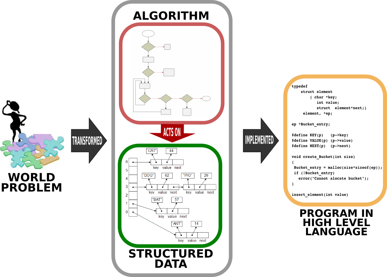
Fig. 2.1.1 Solving a world problem with a computer requires first designing how the data is going to be represented and specifying the steps which yield the solution when executed on the data. This design of the solution is then written (implemented) in a programming language to be executed as a program such that, when executed, the program outputs the solution for the world problem. [From: G. Üçoluk, S. Kalkan, Introduction to Programming Concepts with Case Studies in Python, Springer, 2012]

2.2. Algorithm

An algorithm is a step-by-step procedure that, when executed, leads to an output for the input we provided. If the procedure was correct, we expect the output to be the desired output, i.e. the solution we wanted for the algorithm to compute.

Algorithms can be thought of as recipes for cooking. This analogy makes sense since we would define a recipe as a step-by-step procedure for cooking something: Each step performs a little action (cutting, slicing, stirring etc.) that brings us closer to the outcome, the meal.

This is exactly the case in algorithms as well: At each step, we make a small progress towards the solution by performing a small computation (e.g. adding numbers, finding the minimum of a set of real numbers etc.). The only difference with cooking is that each step needs to be understandable by the computer; otherwise, it is not an algorithm.

The origins of the world ‘algorithm’ The word ‘algorithm’ comes from the Latin word algorithmi, which is the Latinized name of Al-Khwarizmi. Al-Khwarizmi was a Persian Scientist who has written a book on algebra titled “The Compendious Book on Calculation by Completion and Balancing” during 813–833 which presented the first systematic solution of linear and quadratic equations. His contributions established algebra, which stems from his method of “al-jabr” (meaning “completion” or “rejoining”). The reason the world algorithm is attributed to Al-Khwarizmi is because he proposed systematic methods for solving equations using sequences of well-defined instructions (e.g. “take all variables to the right. divide the coefficients by the coefficient of x…”) – i.e. using what we call today as algorithms.

Fig. 2.2.1 Muhammad ibn Musa al-Khwarizmi (c. 780 – c. 850)

** Are algorithms the same thing as programs? **

It is very natural to confuse algorithms with programs as they are both step-by-step procedures. However, algorithms can be studied and they were invented long before there were computers or programming languages. We can design and study algorithms without using computers with just a pen and paper. A program, on the other hand, is just an implementation of an algorithm in a programming language. In other words, algorithms are designs and programs are the written forms of these designs in programming languages.

2.2.1. How to write algorithms

As we have discussed above, before programming our solution, we first need to design it. While designing an algorithm, we generally use two mechanisms:

1. Pseudo-codes. Pseudo-codes are natural language descriptions of the steps that need to be followed in the algorithm. It is not as specific or restricted as a programming language but it is not as free as the language we use for communicating with other humans: A pseudo-code should be composed of precise and feasible steps and avoid ambiguous descriptions.

Here is an example pseudo-code:

Algorithm 1. Calculate the average of numbers provided by the user.

Input: N -- the count of numbers
Output: The average of N numbers to be provided
Step 1: Get how many numbers will be provided and store that in N
Step 2: Create a variable named Result with initial value 0
Step 3: Execute the following step N times:
Step 4:    Get the next number and add it to Result
Step 5: Divide Result by N to obtain the average

2. Flowcharts. As an alternative to pseudocodes, we can use flowcharts while designing algorithms. Flowcharts are diagrams composed of small computational elements that describe the steps of the algorithm. An example in Fig. 2.2.2 illustrates what kind of elements are used and how they are brought together to describe an algorithm.

Flowcharts can be more intuitive to work with. However, for complex algorithms, flowcharts can get very large and prohibitive to work with.

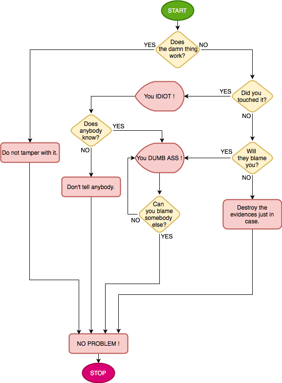
Fig. 2.2.2 Flowcharts describe relationships by using basic geometric symbols and arrows. The program start or end is depicted with an oval. A rectangular box denotes a simple action or status. Decision making is represented by a diamond and a parallelogram of the Input/Output process. A silhouette of a TV tube means displaying a message. The Internet is portrayed as a cloud.

2.2.2. How to compare algorithms

If two algorithms find the same solution, are they of the same quality? For a second, recall a game we used to play when we were in primary school: “Guess My Number”.

The rule is as follows: There is a setter and a guesser. The setter sets a number from 1 to 1000 which s/he does not tell. The guesser has to find this number. At each turn of the game, the guesser can propose any number from 1 to 1000. The setter answers by one of following:

• HIT: The guesser found the number.

• LESSER: The hidden number is less than the proposed one.

• GREATER: The hidden number is greater than the proposed one.

In how many turns the number is found is recorded. The guesser and the setter switch. This goes on for some agreed count of rounds. Whoever has a lower total count of turns wins.

Many of you have played this game and certainly have observed that there are three categories of children:

1. Random guessers: Worst category. Usually they cannot keep track of the answers and just based on the last answer, they randomly utter a number that comes to their mind. Quite possibly they repeat themselves.

2. Sweepers: They start at either 1 or 1000, and then systematically increase or decrease their proposal, e.g.:

   • -is it 1000? Answer: LESSER

   • -is it 999? Answer: LESSER

   • -is it 998? Answer: LESSER

   … and so on. Certainly at some point such players do get a HIT. There is a group which decreases the number by two or three as well. With a first GREATER reply, they start to increment by one.

3. Middle seekers: Keeping a possible lower and a possible upper value based on the reply they got, at every stage they propose the number just in the middle of lower and upper values, e.g.:

   • -is it 500? Answer: LESSER

   • -is it 250? Answer: LESSER

   • -is it 125? Answer: GREATER

   • -is it 187? (which was (125+250)/2) Answer: GREATER

   • … and so on.

All three categories actually adopt different algorithms, which will find the answer in the end. However, as you may have realised even as you were a child, the first group performs the worst, then comes the second group. The third group, if they do not make mistakes, is unbeatable.

In other words, algorithms that aim to solve the same problem may not be of the same “quality”: Some perform better. This is the case for all algorithms and one of the challenges in Computer Science is to find “better” algorithms. But, what is “better”? Is there a quantitative measure for “better”ness? The answer is yes.

Let us look at this in the child game described above. First consider the last group’s algorithm (the middle seekers). At every turn, this kind of seeker narrows down the search space by a factor of 1/2. Starting with 1000 numbers, the search space is reduced as follows: \(1000\), \(1000/2\), \(1000/2^2\), … So, in the worst case, it will take \(m\) turns until \(1000/2^m\) gets down to 1 (the one remaining number, which has to be the hidden number). In other words, in the worst case, \(1000/2^m=1\) and from this we can derive \(m=\log_2(1000)\). For 1000, this means approximately \(m=10\) turns. If we double the range, \(m\) would change only by 1 (yes, think about it, only 11 turns).

We call such an algorithm of “order log(n)” or more technically, \(\cal{O}(\log(n))\). In our case 1000 determines the ‘size’ of the problem. This is symbolized with \(n\). \(\cal{O}(\log(n))\) is the quantitative information about the algorithm which signifies that the solution time is proportional to \(\log(n)\). This information about an algorithm is named as complexity.

What about the sweepers algorithm for the problem above? In the worst case, the sweeper would ask a question 1000 times (the correct number is at the other end of the sequence). If the size (1000 in our case) is symbolized with \(n\), then it will take a time proportional to \(n\) to reach the solution. In other words this algorithm’s complexity is \(\cal{O}(n)\).

Certainly the algorithm that has \(\cal{O}(\log(n))\) is better than the one with \(\cal{O}(n)\), which is illustrated in Fig. 2.2.3. In other words, an \(\cal{O}(\log(n))\) algorithm requires less number of steps and is likely to run faster than the one with \(\cal{O}(n)\) complexity.

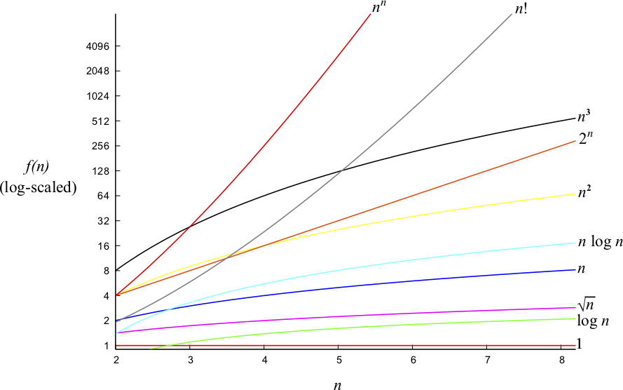
Fig. 2.2.3 A plot of various complexities.

2.3. Data Representation

The other crucial component of our solutions to world problems is the data representation, which deals with encoding the information regarding the problem in a form that is most suitable for our algorithm.

If our problem is the calculation of the average of grades in a class, then before implementing our solution, we need to determine how we are going to represent (encode) the grades of students. This is what we are going to determine in the ‘data representation’ part of our solution and to discuss in Chapter 3.

2.4. The World of Programming Languages

Since the advent of computers, many programming languages have been developed with different designs and levels of complexity. In fact, there are about 700 programming languages - see, e.g. the list of programming languages - that offer different abstraction levels (hiding the low-level details from the programmer) and computational benefits (e.g. providing built-in rule-search engine).

In this section, we will give a flavour of programming languages in terms of abstraction levels (low-level vs. high-level – see Fig. 2.4.1) as well as the computational benefits they provide.

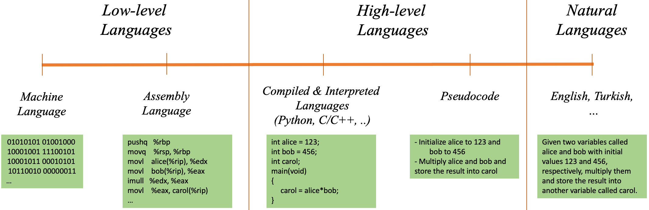
Fig. 2.4.1 The spectrum of programming languages, ranging from low-level languages to high-level languages and natural languages.

2.4.1. Low-level Languages

In the previous chapter, we introduced the concept of machine code program. A machine code program is an aggregate of instructions and data, all being represented in terms of zeros (0) and ones (1). A machine code is practically unreadable and very burdensome to create, as we have seen before and illustrated below:

01010101 01001000 10001001 11100101 10001011 00010101 10110010 00000011
00100000 00000000 10001011 00000101 10110000 00000011 00100000 00000000
00001111 10101111 11000010 10001001 00000101 10111011 00000011 00100000
00000000 10111000 00000000 00000000 00000000 00000000 11001001 11000011
...
11001000 00000001 00000000 00000000  00000000 00000000

To overcome this, assembly language and assemblers were invented. An assembler is a machine code program that serves as a translator from some relatively more readable text, the assembly program, into machine code. The key feature of an assembler is that each line of an assembly program corresponds exactly to a single machine code instruction. As an example, the binary machine code above can be written in an assembly language as follows:

main:
       pushq   %rbp
       movq    %rsp, %rbp
       movl    alice(%rip), %edx
       movl    bob(%rip), %eax
       imull   %edx, %eax
       movl    %eax, carol(%rip)
       movl    $0, %eax
       leave
       ret
alice:
       .long   123
bob:
       .long   456

Pros of assembly:

• Instructions and registers have human recognizable mnemonic words associated. Like integer addition instruction being ADDI, for example.

• Numerical constants can be written down in human readable, base-10 format, the assembler does the conversion to internal format.

• Implements naming of memory positions that hold data. In other words, assembly has a primitive implementation of the variable concept.

Cons of assembly:

• No arithmetic or logical expressions.

• No concept of functions.

• No concept of statement grouping.

• No concept of data containers.

2.4.2. High-level Languages

To overcome the limitations of binary machine codes and the assembly language, more capable Programming Languages were developed. We call these languages High-level languages. These languages hide the low-level details of the computer (and the CPU) and allow a programmer to write code in a more human-readable form.

A high-level programming language (or an assembly language) is defined, similar to a natural language, by syntax (a set of grammar rules governing how to bring together words) and semantics (the meaning – i.e. what is meant by the sequences of words in the syntax) associated for the syntax. The syntax is based on keywords from a human language (due to historical reasons, English). Using human-readable keywords ease comprehension.

The following example is a program expressed in Python that asks for a Fahrenheit value and prints its conversion into Celsius:

Fahrenheit =  input("Please Enter Fahrenheit value:")
print("Celsius equivalent is:", (Fahrenheit − 32) * 5/9)

Here input and print are keywords of the language. Their semantics is self explanatory. Fahrenheit is a naming we have chosen for a variable that will hold the input value.

High-level languages (HL-languages from now on) implement many concepts which are not present at the machine code programming level. Most outstanding features are:

• human readable form of numbers and strings (like decimal, octal, hexadecimal representations for numbers),

• containers (automatic allocation for places in the memory to hold, access and name data),

• expressions (calculation formulas based on operators which have precedences the way we are used to from mathematics),

• constructs for repetitive execution (conditional re-execution of code parts),

• functions,

• facilities for data organization (ability to define new data types based on the primitive ones, organizing them in the memory in certain layouts).

2.4.3. Implementing with a High-level Language: Interpreter vs. Compiler

We can implement our solution in a high-level programming language in two manners:

1. Compilative Approach. In this approach, a translator, called compiler, takes a high-level programming language program as input and converts all actions in the program into a machine code program (Fig. 2.4.2). The outcome is a machine code program that can be run any time (by asking the OS to do so) and does the job described in the high-level language program.

Conceptually this is correct, but actually, this schema has another step in-the-loop. The compiler produces an almost complete machine code with some holes in it. These holes are about the parts of the code which is not actually coded by the programmer, but filled in from a pre-created machine code library (it is actually named as library). A program, named linker fills those holes. The linker knows about the library and patches in the parts of the code that are referenced by the programmer.

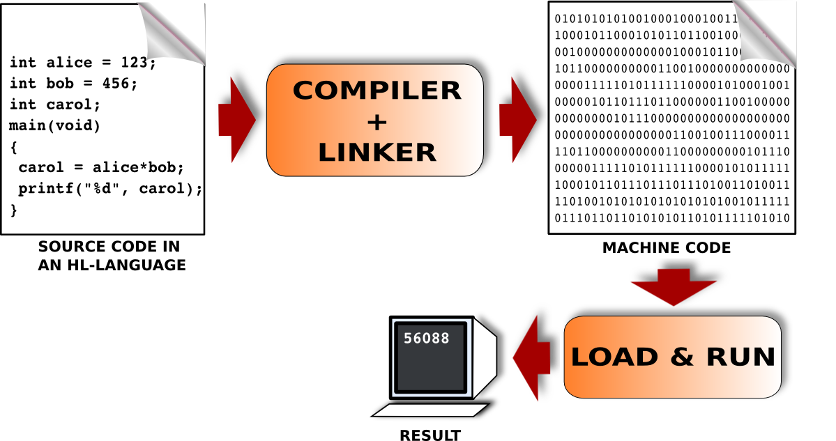
Fig. 2.4.2 A program code in a high-level language is first translated into machine understandable binary code (machine code) which is then loaded and executed on the machine to obtain the result. [From: G. Üçoluk, S. Kalkan, Introduction to Programming Concepts with Case Studies in Python, Springer, 2012]

2. Interpretive Approach. In this approach, a machine code program, named as interpreter, when run, inputs and processes the high-level program line by line (Fig. 2.4.3). After taking a line as input, the actions described in the line are immediately executed; if the action is printing some value, the output is printed right away; if it is an evaluation of a mathematical expression, all values are substituted and at that very point-in-time, the expression is evaluated to calculate the result. In other words, any action is carried out immediately when the interpreter comes to its line in the program. In practice, it is always possible to write down the program lines into a file, and make the interpreter read the program lines one by one from that file as well.

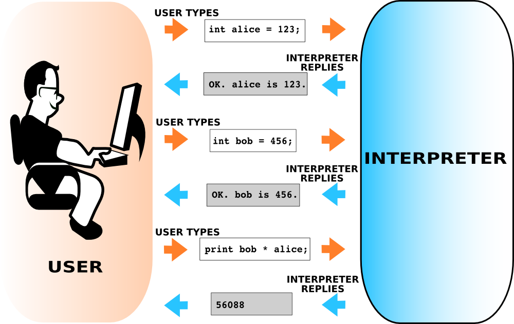
Fig. 2.4.3 Interpreted languages (e.g. Python) come with interpreters that process and evaluate each action (statement) from the user on the run and returns an answer. [From: G. Üçoluk, S. Kalkan, Introduction to Programming Concepts with Case Studies in Python, Springer, 2012]

Which approach is better?

Both approaches have their benefits. When a specific task is considered, compilers generate fast executing machine codes compared to the same task being carried out by an interpreter. On the other hand compilers are unpleasant when trial-and-errors are possible while developing the solution. Interpreters, on the other hand, allow making small changes and the programmer receives immediate responses, which makes it easier to observe intermediate results and adjust the algorithm accordingly. However, interpreters are slower since they involve an interpretation component while running the code. Sometimes this slowness is by a factor of 20. Therefore, the interpretive approach is good for quick implementations whereas using a compiler is good for computation-intense big projects or time-tight tasks.

2.4.4. Programming-language Paradigms

As we mentioned before, there are more than 700 programming languages. Certainly some are for academic purposes and some did not gain any popularity. But there are about 20 programming languages which are commonly used for writing programs. How do we choose one when implementing our solution?

Picking a particular programming language is not just a matter of taste. During the course of the evolution of the programming languages, different strategies or world views about programming have also developed. These world views are reflected in the programming languages.

For example, one world view regards the programming task as transforming some initial data (the initial information that defines the problem) into a final form (the data that is the answer to that problem) by applying a sequence of functions. From this perspective, writing a program consists of defining some functions which are then used in a functional composition; a composition which, when applied to some initial data, yields the answer to the problem.

This concept of world views are coined as programming paradigms. The Oxford dictionary defines the word paradigm as follows:

paradigm \(|\)’parǝ,dïm\(|\)

noun

A world view underlying the theories and methodology of a particular scientific subject.

Below is a list of some major paradigms:

• Imperative: Is a paradigm where programming statements and their composition directly map to the machine code segments, so that the whole machine code is covered.

• Functional: In this paradigm, solving a programming task is to construct a group of functions so that their ‘functional composition’ acting on the initial data produces the solution.

• Object oriented: In this paradigm the compulsory separation (due to the von Neumann architecture) of algorithm from data is lifted, and algorithm and data are reunited under an artificial computational entity: the object. An object has algorithmic properties as well as data properties.

• Logical-declarative: This is the most contrasting view compared to the imperative paradigm. The idea is to represent logical and mathematical relations among entities (as rules) and then ask an inference engine for a solution that satisfies all rules. The inference engine is a kind of ‘prover’, i.e. a program, that is constructed by the inventor of the logical-declarative programming language.

• Concurrent: A paradigm where independent computational entities work towards the solution of a problem. For problems that can be solved by a divide-and-conquer strategy, this paradigm is very suitable.

• Event driven: This paradigm introduces the concept of events into programming. Events are assumed to be asynchronous and they have ‘handlers’, i.e. programs that carry out the actions associated with a particular event. Programming graphical user interfaces (GUIs) is usually performed using event-driven languages: An event in a GUI is generated e.g. when the user clicks the “Close” button, which triggers the execution of a handler function that performs the associated closing action.

In contrary to the layman programmers’ assumption, these paradigms are not mutually exclusive. Many paradigms can very well co-exist in a programming language together. At a meta level, we can call them ‘orthogonal’ to each other. This is why we have so many programming languages around. A language can provide imperative as well as functional and object-oriented constructs. Then it is up to the programmer to blend them in his or her particular program. As it is with many ‘world views’ among humans, in the field of programming, fanaticism exists too. You can meet individuals that do only functional programming or object-oriented programming. We better consider them outliers.

Python, the subject language of this book, supports strongly the imperative, functional and object-orient paradigms. It also provides some functionality in other paradigms by some modules.

2.5. Introducing Python

After having provided background on the world of programming, let us introduce Python: Although it is widely known to be a recent programming language, Python’s design, by Guido van Rossum, dates back to 1980s, as a successor of the ABC programming language. The first version was released in 1991 and with the second version released in 2000, it started gaining a wider interest from the community. After it was chosen by some big IT companies as the main programming language, Python became one of the most popular programming languages.

An important reason for Python’s wide acceptance and use is its design principles. By design, Python is a programming language that is easier to understand and to write but at the same time powerful, functional, practical and fun. This has deep roots in its design philosophy (a.k.a. The Zen of Python):

“Beautiful is better than ugly. Explicit is better than implicit. Simple is better than complex. Complex is better than complicated. Readability counts. [… there are 14 more]”

Python is multi-paradigm programming language, supporting imperative, functional and object-oriented paradigms, although the last one is not one of its strong suits, as we will see in Chapter 7. Thanks to its wide acceptance especially in the open-source communities, Python comes with or can be extended with an ocean of libraries for practically solving any kind of task.

The word ‘python’ was chosen as the name for the programming language not because of the snake species python but because of the comedy group Monty Python. While van Possum was developing Python, he read the scripts of Monty Python’s Flying Circus and thought ‘python’ was “short, unique and mysterious” for the new language. To make Python more fun to learn, earlier releases heavily used phrases from Monty Python in example programming codes.

With version 3.9 being released in October 2020 as the latest version, Python is one of the most popular programming languages in a wide spectrum of disciplines and domains. With an active support from the open-source community and big IT companies, this is not likely to change in the near future. Therefore, it is in your best interest to get familiar with Python if not excel in it.

This is how the Python interpreter looks like at a Unix terminal:

$ python3
Python 3.8.5 (default, Jul 21 2020, 10:48:26)
[Clang 11.0.3 (clang-1103.0.32.62)] on darwin
Type "help", "copyright", "credits" or "license" for more information.
>>>

The three symbols >>> indicate that the interpreter is ready to collect our computational demands, e.g.:

>>> 21+21
42

where we asked what was 21+21 and Python responded with 42, which is one small step for a man but one giant leap for mankind.

2.6. Important Concepts

We would like our readers to have grasped the following crucial concepts and keywords from this chapter:

• How we solve problems using computers.

• Algorithms: What they are, how we write them and how we compare them.

• The spectrum of programming languages.

• Pros and cons of low-level and high-level languages.

• Interpretive vs. compilative approach to programming.

• Programming paradigms.

2.7. Further Reading

• The World of Programming chapter available at: https://link.springer.com/chapter/10.1007/978-3-7091-1343-1_1

• Programming Languages:

  • For a list of programming languages: http://en.wikipedia.org/wiki/Comparison_of_programming_languages

  • For a comparison of programming languages: http://en.wikipedia.org/wiki/Comparison_of_programming_languages

  • For more details: Daniel P. Friedman, Mitchell Wand, Christopher Thomas Haynes: Essentials of Programming Languages, The MIT Press 2001.

• Programming Paradigms:

  • Introduction: http://en.wikipedia.org/wiki/Programming_paradigm

  • For a detailed discussion and taxonomy of the paradigms: P. Van Roy, Programming Paradigm for Dummies: What Every Programmer Should Know, New Computational Paradigms for Computer Music, G. Assayag and A. Gerzso (eds.), IRCAM/Delatour France, 2009 http://www.info.ucl.ac.be/~pvr/VanRoyChapter.pdf

  • Comparison between Paradigms: http://en.wikipedia.org/wiki/Comparison_of_programming_paradigms

2.8. Exercise

• Draw the flowchart for the following algorithm:

Step 1: Get a list of N numbers in a variable named Numbers
Step 2: Create a variable named Sum with initial value 0
Step 3: For each number i in Numbers, execute the following line:
Step 4:     if i > 0: Add i to Sum
Step 5:     if i < 0: Add the square of i to Sum
Step 5: Divide Sum by N

• What is the complexity of Algorithm 1 (in Section 2.2)?

• What is the complexity of the following algorithm?

Step 1: Get a list of N numbers in a variable named Numbers
Step 2: Create a variable named Mean with initial value 0
Step 3: For each number i in Numbers, execute the following line:
Step 4:     Add i to Mean
Step 5: Divide Mean by N
Step 6: Initialize a variable named Std with value 0
Step 7: For each number i in Numbers, execute the following line:
Step 8:    Add the square of (i-Mean) to Std
Step 9: Divide Std by N and take its square root

• Assuming that a step of an algorithm takes 1 second, fill in the following table for different algorithms for different input sizes (\(n\)):

Input Size	\(\cal{O}(\log n)\)	\(\cal{O}(n)\)	\(\cal{O}(n \log n)\)	\(\cal{O}(n^2)\)	\(\cal{O}(n^3)\)	\(\cal{O}(2^n)\)	\(\cal{O}(n^n)\)
\(n=10^2\)
\(n=10^3\)
\(n=10^4\)
\(n=10^5\)

• Assume that we have a parser than can process and parse natural language descriptions (without any syntactic restrictions) for programming a computer. Given such a parser, do you think we would use natural language to program computers? If no, why not?

• For each situation below, try to identify which paradigm is more suitable compared to the others:

• Writing a program which should take an image as input, an RGB color value and find all pixels in the image that match the given color.

• Writing a theorem proving program.

• Writing the auto pilot program flying an airplane.

• Writing a document editing program as an alternative to Microsoft Word.